Physics Formulae/Electromagnetism Formulae

Lead Article: Tables of Physics Formulae

This article is a summary of the laws, principles, defining quantities, and useful formulae in the analysis of Electromagnetism.

Laws of Electromagnetism

Maxwell's Equations

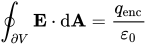
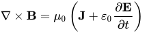
Below is the set in the differential and integral forms, each form is found to be equivalant by use of vector calculus. There are many ways to formulate the laws using scalar/vector potentails, tensors, geometric algebra, and numerous variations using different field vectors for the electric and magnetic fields.

Name	Differential form	Integral form
Gauss's law	$\mathrm{\nabla }\cdot 𝐄=\frac{\rho }{{\epsilon }_0}$	${\oint }_{\partial V}𝐄\cdot \mathrm{d}𝐀=\frac{q_{\mathrm{e}\mathrm{n}\mathrm{c}}}{{\epsilon }_0}$
Gauss's law for Magnetism	$\mathrm{\nabla }\cdot 𝐁=\mathrm{𝟎}$	${\oint }_{\partial V}𝐁\cdot \mathrm{d}𝐀=0$
Maxwell–Faraday Law (Faraday's law of induction)	$\mathrm{\nabla }\times 𝐄=-\frac{\partial 𝐁}{\partial t}$	$V=-{\oint }_{\partial S}𝐄\cdot \mathrm{d}𝐥=-{\oint }_{\partial S}\frac{\partial 𝐁}{\partial t}\cdot \mathrm{d}𝐀$
Maxwell-Ampère Circuital law (Ampere's Law with Maxwell's correction)	$\mathrm{\nabla }\times 𝐁={\mu }_0(𝐉+{\epsilon }_0\frac{\partial 𝐄}{\partial t})$	${\oint }_{\partial S}𝐁\cdot \mathrm{d}𝐥={\mu }_0{\oint }_{\partial S}(𝐉+{\epsilon }_0\frac{\partial 𝐄}{\partial t})\cdot \mathrm{d}𝐀$
Lorentz Electromagnetic Force Law	$𝐅=q_e(𝐄+𝐯\times 𝐁)$

The Field Vectors

Central to electromagnetism are the electric and magnetic field vectors. Often for free space (vacumm) only the familiar E and B fields need to be used; but for matter extra field vectors D, P, H, and M must be used to account for the electric and magnetic dipole incluences throughout the media (see below for mathematical definitions).

The electric field vectors are related by:	$𝐃={ϵ}_0𝐄+𝐏$
The magnetic field vectors are related by:	$𝐁={\mu }_0(𝐇+𝐌)$

Interpretation of the Field Vectors

Intuitivley;

— the E and B (electric and magnetic flux densities) fields are the easiest to interpret; field strength is propotional to the amount of flux though cross sections of surface area, i.e. strength as a cross-section density.

— the P and M (electric polarization and magnetization respectivley) fields are related to the net polarization of the dipole moments thoughout the medium, i.e. how well they respond to an external field, and how the orientation of the dipoles can retain (or not) the field they set up in response to the external field.

— the D and H (electric displacement and magnetic intensity field) fields are the least clear to understand physically; they are introduced for convenient thoretical simplifications, but one could imagine they relate to the strength of the field along the flux lines, strength as a linear density along flux lines.

Hypothical Magnetic Monopoles

— As far as is known, there are no magnetic monopoles in nature, though some theories predict they could exist.

— The approach to introduce monopoles in equations is to define a magnetic pole strength, magnetic charge, or monopole charge (all synonomous), treating poles analogously to the electric charges.

— One pole would be north N (numerically positive by convention), the other south S (numerically negative). There are two units which can be used from the SI system for pole strength.

— Pole srength can be quantified into densities, currents and current densities, as electric charge is in the previous table, exactly in the same way.

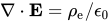
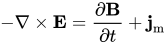
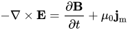
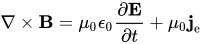
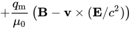
Maxwell's Equations would become one of the columns in the table below, at least theoretically. Subscripts e are electric charge quantities; subscripts m are magnetic charge quantities.

Name	Weber (Wb) Convention	Ampere meter (A m) Convention
Gauss's Law	$\mathrm{\nabla }\cdot 𝐄={\rho }_{\mathrm{e}}/{ϵ}_0$	$\mathrm{\nabla }\cdot 𝐄={\rho }_{\mathrm{e}}/{ϵ}_0$
Gauss's Law for magnetism	$\mathrm{\nabla }\cdot 𝐁={\rho }_{\mathrm{m}}$	$\mathrm{\nabla }\cdot 𝐁={\mu }_0{\rho }_{\mathrm{m}}$
Faraday's Law of induction	$-\mathrm{\nabla }\times 𝐄=\frac{\partial 𝐁}{\partial t}+{𝐣}_{\mathrm{m}}$	$-\mathrm{\nabla }\times 𝐄=\frac{\partial 𝐁}{\partial t}+{\mu }_0{𝐣}_{\mathrm{m}}$
Ampère's Law	$\mathrm{\nabla }\times 𝐁={\mu }_0{ϵ}_0\frac{\partial 𝐄}{\partial t}+{\mu }_0{𝐣}_{\mathrm{e}}$	$\mathrm{\nabla }\times 𝐁={\mu }_0{ϵ}_0\frac{\partial 𝐄}{\partial t}+{\mu }_0{𝐣}_{\mathrm{e}}$
Lorentz force equation	$𝐅=q_{\mathrm{e}}(𝐄+𝐯\times 𝐁)+$ $+\frac{q_{\mathrm{m}}}{{\mu }_0}(𝐁-𝐯\times (𝐄/c^2))$	$𝐅=q_{\mathrm{e}}(𝐄+𝐯\times 𝐁)+$ $+q_{\mathrm{m}}(𝐁-𝐯\times (𝐄/c^2))$

They are consistent if no magnetic monopoles, since monopole quantities are then zero and the equations reduce to the original form of Maxwell's equations.

Pre-Maxwell Laws

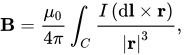
These laws are not fundamental anymore, since they can be derived from Maxwell's Equations. Coulomb's Law can be found from Gauss' Law (electrostatic form) and the Biot-Savart Law can be deduced from Ampere's Law (magnetostatic form). Lenz' Law and Faraday's Law can be incorperated into the Maxwell-Faraday equation. Nonetheless they are still very effective for simple calculations, especially for highly symmetrical problems.

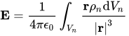
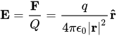
Coulomb's Law	$𝐄=\frac{𝐅}{Q}=\frac{q}{4\pi {ϵ}_0{\left|𝐫\right|}^2}\widehat{𝐫}$ For a non uniform charge distribution, this becomes: $𝐄=\frac{1}{4\pi {ϵ}_0}{\int }_{V_n}\frac{𝐫{\rho }_n\mathrm{d}{V}_n}{{\left|𝐫\right|}^3}$
Biot-Savart Law	$𝐁=\frac{{\mu }_0}{4\pi }{\int }_C\frac{I(\mathrm{d}𝐥\times 𝐫)}{{\left|𝐫\right|}^3},$
Lenz's law	Induced current always opposes its cause.

Electric Quantities

Electric Charge and Current

Quantity (Common Name/s)	(Common) Symbol/s	Defining Equation	SI Units	Dimension
Elementary Charge Quantum	$e$		C = A s	[I][T]
Quantized Electric Charge	q	$q=ne$	C = A s	[I][T]
Electric Charge (any amount)	$q$		C = A s	[I][T]
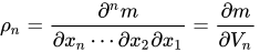
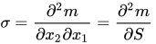
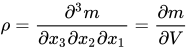
Electric charge density of dimension n ($V_n$ = n-space) n = 1 for linear mass density, n = 2 for surface mass density, n = 3 for volume mass density, etc	linear charge density $\lambda$, surface charge density $\sigma$, volume charge density $\rho$, no general symbol for any dimension	n-space charge density: ${\rho }_n=\frac{{\partial }^{n}m}{\partial x_n\cdots \partial x_2\partial x_1}=\frac{\partial m}{\partial V_n}$ special cases are: $\lambda =\frac{\partial m}{\partial x}$ $\sigma =\frac{{\partial }^{2}m}{\partial x_2\partial x_1}=\frac{{\partial }^{2}m}{\partial S}$ $\rho =\frac{{\partial }^{3}m}{\partial x_3\partial x_2\partial x_1}=\frac{\partial m}{\partial V}$	C m-n	[I][T][L]-n
Total descrete charge	$Q$	$Q=\sum _i{q}_i$	C	[I][T]
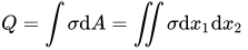
Total continuum charge	$Q$	n-space charge density $Q=\int {\rho }_n{\mathrm{d}}^{n}x=\int \cdots \int \int {\rho }_n\mathrm{d}{x}_1\mathrm{d}{x}_2\cdots \mathrm{d}{x}_n$ special cases are: $Q=\int \lambda \mathrm{d}x$ $Q=\int \sigma \mathrm{d}A=\iint \sigma \mathrm{d}{x}_1\mathrm{d}{x}_2$ $Q=\int \rho \mathrm{d}V=\iiint \rho \mathrm{d}{x}_1\mathrm{d}{x}_2\mathrm{d}{x}_3$	C	[I][T]
Capacitance	$C$	$C=\frac{\partial q}{\partial V}$	F = C V-1
Electric Current	$I$	$I=\frac{\mathrm{d}q}{\mathrm{d}t}$	A	[I]
Current Density	$𝐉$	$𝐉=\widehat{𝐀}\frac{\partial I}{\partial A}$	A m-2	[I][L]-2
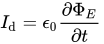
Displacement current	$I_{\mathrm{d}}$	$I_{\mathrm{d}}={ϵ}_0\frac{\partial {\Phi }_E}{\partial t}$	A	[I]
Charge Carrier Drift Speed	${𝐯}_d$		m s-1	[L][T]-1

Electric Fields

Quantity (Common Name/s)	(Common) Symbol/s	Defining Equation	SI Units	Dimension
Electric Field, Field Strength, Flux Density, Potential Gradient	$𝐄$	$𝐄=𝐅/q$	N C-1 = V m-1	[M][L][T]-3[I]-1
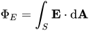
Electric Flux	${\Phi }_E$	${\Phi }_E={\int }_S𝐄\cdot \mathrm{d}𝐀$	N m2 C-1	[M][L]3[T]-3[I]-1
Electric Permittivity	$ϵ$	$ϵ={ϵ}_{\mathrm{r}}{ϵ}_0$	F m-1
Dielectric constant, Relative Permittivity	${ϵ}_{\mathrm{r}}$		F m-1
Electric Displacement Field	$𝐃$	$𝐃=\frac{𝐄}{ϵ}$	C m-2	[I][T][L]-2
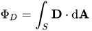
Electric Displacement Flux	${\Phi }_D$	${\Phi }_D={\int }_S𝐃\cdot \mathrm{d}𝐀$	C	[I][T]
Electric Dipole Moment vector	$𝐩$	$𝐩=2q𝐚$ $𝐚$ is the charge separation directed from -ve to +ve charge	C m	[I][T][L]
Electric Polarization	$𝐏$	$𝐏=\frac{\partial ⟨𝐩⟩}{\partial V}$	C m-2	[I][T][L]-2
Absolute Electric Potential relative to point $r_0$ Theoretical: $r_0=\mathrm{\infty }$ Practical: $R_0=R_{\mathrm{e}\mathrm{a}\mathrm{r}\mathrm{t}\mathrm{h}}$ (Earth's radius)	$\varphi ,V$	$V=-\frac{W_{\mathrm{\infty }r}}{q}=-\frac{1}{q}{\int }_{\mathrm{\infty }}^r𝐅\cdot \mathrm{d}𝐫=-{\int }_{r_1}^{r_2}𝐄\cdot \mathrm{d}𝐫$	V = J C-1
Electric Potential Difference	$\mathrm{\Delta }V$	$\Delta V=-\frac{\Delta W}{q}=-\frac{1}{q}{\int }_{r_1}^{r_2}𝐅\cdot \mathrm{d}𝐫=-{\int }_{r_1}^{r_2}𝐄\cdot \mathrm{d}𝐫$
Electric Potential Energy	$U$	$U=-W$	J	[M][L]2[T]2

Magnetic Quantities

Quantity (Common Name/s)	(Common) Symbol/s	Defining Equation	SI Units	Dimension
Magnetic Field, Field Strength, Flux Density, Induction Field	$𝐁$	$𝐅=q(𝐯\times 𝐁)$	T = N A-1 m-1
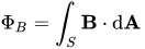
Magnetic Flux	${\Phi }_B$	${\Phi }_B={\int }_S𝐁\cdot \mathrm{d}𝐀$	Wb = T m-2
Magnetic Permeability	$\mu$	$\mu ={\mu }_{\mathrm{r}}{\mu }_0$	H m-1
Relative Permeability	${\mu }_{\mathrm{r}}$		H m-1
Magnetic Field Intensity, (also confusingly the field strength)	$𝐇$	$𝐇=\frac{𝐁}{\mu }$
Magnetic Dipole Moment vector	$𝐦$	$𝐦=NI𝐀$ N is the number of turns of conductor	A m2	[I][L]2
Magnetization	$𝐌$	$𝐌=\frac{\partial ⟨𝐦⟩}{\partial V}$
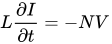
Self Inductance	$L$	Two equivalent definitions are in fact possible: $L=N\frac{\partial \Phi }{\partial I}$ $L\frac{\partial I}{\partial t}=-NV$	H = Wb A-1
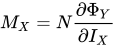
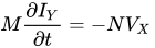
Mutual Inductance	$M$	Again two equivalent definitions are in fact possible: $M_X=N\frac{\partial {\Phi }_Y}{\partial I_X}$ $M\frac{\partial I_Y}{\partial t}=-N{V}_X$ X,Y subscripts refer to two conductors mutually inducing voltage/ linking magnetic flux though each other	H = Wb A-1

Electric Fields

Electrostatic Fields

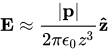
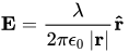
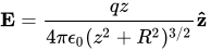
Common corolaries from Couloumb's and Gauss' Law (in turn corolaries of Maxwell's Equations) for uniform charge distributions are summarized in the table below.

Uniform Electric Field accelerating a charged mass	$a=\frac{qE}{m}$
Point Charge	$𝐄=\frac{q}{4\pi {ϵ}_0{\left|𝐫\right|}^2}\widehat{𝐫}$
At a point in a local array of Point Charges	$𝐄=\sum {𝐄}_i=\frac{1}{4\pi {ϵ}_0}\sum _i\frac{q_i}{{|{𝐫}_i-𝐫|}^2}{\widehat{𝐫}}_i$
Electric Dipole	$𝐄\approx \frac{\left|𝐩\right|}{2\pi {ϵ}_0{z}^3}\widehat{𝐳}$ $\left|𝐫\right|>>\left|𝐚\right|$
Line of a Charge	$𝐄=\frac{\lambda }{2\pi {ϵ}_0\left|𝐫\right|}\widehat{𝐫}$
Charged Ring	$𝐄=\frac{qz}{4\pi {ϵ}_0(z^2+R^2{)}^{3/2}}\widehat{𝐳}$
Charged Conducting Surface	$𝐄=\frac{\sigma }{{ϵ}_0}\widehat{𝐧}$
Charged Insulating Surface	$𝐄=\frac{\sigma }{2{ϵ}_0}\widehat{𝐧}$
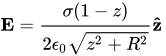
Charged Disk	$𝐄=\frac{\sigma (1-z)}{2{ϵ}_0\sqrt{z^2+R^2}}\widehat{𝐳}$
Outside Spherical Shell r>=R	$𝐄=\frac{q}{4\pi {ϵ}_0{\left|𝐫\right|}^2}\widehat{𝐫}$
Inside Spherical Shell r<R	$𝐄=\mathrm{𝟎}$
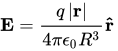
Uniform Charge r<=R	$𝐄=\frac{q\left|𝐫\right|}{4\pi {ϵ}_0{R}^3}\widehat{𝐫}$
Electric Dipole Potential Energy in a uniform Electric Eield	$U=-𝐩\cdot 𝐄$
Torque on an Electric Dipole in a uniform Electric Eield	$𝝉=𝐩\times 𝐄$
Electric Field Energy Density Linear media (constant $ϵ$ throughout)	$u=\frac{ϵE^2}{2}$

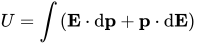
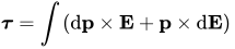
For non-uniform fields and electric dipole moments, the electrostatic torque and potential energy are:

$U=\int (𝐄\cdot \mathrm{d}𝐩+𝐩\cdot \mathrm{d}𝐄)$ $𝝉=\int (\mathrm{d}𝐩\times 𝐄+𝐩\times \mathrm{d}𝐄)$

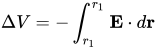
Electric Potential and Electric Field

$\Delta V=-{\int }_{r_1}^{r_1}𝐄\cdot d𝐫$ $\mathrm{\nabla }V=-𝐄$

Electrostatic Potentials

Point Charge	$V=\frac{q}{4\pi {ϵ}_{0}r}$
Pair of Point Charges	$V=\frac{q_1{q}_2}{4\pi {ϵ}_{0}r}$

Electrostatic Capacitances

Parallel Plates	$C=\frac{{ϵ}_{0}A}{d}$
Cylinder	$C=\frac{{ϵ}_{0}2\pi L}{\ln \left|\frac{b}{a}\right|}$
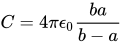
Sphere	$C=4\pi {ϵ}_0\frac{ba}{b-a}$
Isolated Sphere	$C=4\pi {ϵ}_{0}R$
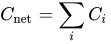
Capacitors Connected in Parallel	$C_{\mathrm{n}\mathrm{e}\mathrm{t}}=\sum _i{C}_i$
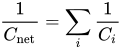
Capacitors Connected in Series	$\frac{1}{C_{\mathrm{n}\mathrm{e}\mathrm{t}}}=\sum _i\frac{1}{C_i}$
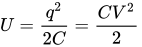
Capacitor Potential Energy	$U=\frac{q^2}{2C}=\frac{C{V}^2}{2}$

Magnetic Fields

Magnetic Forces

Force on a Moving Charge

$𝐅=q𝐯\times 𝐁$

Force on a Current-Carrying Conductor

$𝐅=I𝐥\times 𝐁$

Magnetostatic Fields

Common corolaries from the Biot-Savart Law and Ampere's Law (again corolaries of Maxwell's Equations) for steady (constant) current-carrying configerations are summarized in the table below.

For these types of current configerations, the magnetic field is easily evaluated using the Biot-Savart Law, containing the vector $\mathrm{d}𝐥\times 𝐫$, which is also the direction of the magnetic field at the point evaluated.

For conveinence in the results below, let $𝐛=\mathrm{d}𝐥\times 𝐫$ be a unit binormal vector to $𝐥$ and $𝐫$, so that

$\widehat{𝐛}=\frac{\mathrm{d}𝐥\times 𝐫}{|\mathrm{d}𝐥\times 𝐫|}$

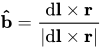
then $\widehat{𝐛}$ also the unit vector for the direction of the magnetic field at the point evaluated.

Hall Effect	$n=\frac{BI}{Vle}$
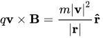
Circulating Charged Particle	$q𝐯\times 𝐁=\frac{m{\left|𝐯\right|}^2}{\left|𝐫\right|}\widehat{𝐫}$
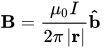
Infinite Line of Current	$𝐁=\frac{{\mu }_{0}I}{2\pi \left|𝐫\right|}\widehat{𝐛}$
Magnetic Field of a Ray	$𝐁=\frac{{\mu }_{0}I}{4\pi \left|𝐫\right|}$
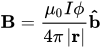
Center of a Circular Arc	$𝐁=\frac{{\mu }_{0}I\varphi }{4\pi \left|𝐫\right|}\widehat{𝐛}$
Infinitley Long Solenoid	$𝐁={\mu }_{0}nI\widehat{𝐛}$
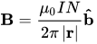
Toroidal Inductors and Transformers	$𝐁=\frac{{\mu }_{0}IN}{2\pi \left|𝐫\right|}\widehat{𝐛}$
Current Carrying Coil	$𝐁=\frac{\mu }{2\pi z^3}\widehat{𝐛}$
Magnetic Dipole Potential Energy in a uniform Magnetic Eield	$U=-𝐦\cdot 𝐁$
Torque on a Magnetic Dipole in a uniform Magnetic Eield	$𝝉=𝐦\times 𝐁$

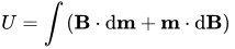
For non-uniform fields and magnetic moments, the magnetic potential energy and torque are:

$U=\int (𝐁\cdot \mathrm{d}𝐦+𝐦\cdot \mathrm{d}𝐁)$ $𝝉=\int (\mathrm{d}𝐦\times 𝐁+𝐦\times \mathrm{d}𝐁)$

Magnetic Energy

Magnetic Energy for Linear Media ($\mu$ constant at all points in meduim)	$U=\frac{L{I}^2}{2}$
Magnetic Energy Density for Linear Media ($\mu$ constant at all points in meduim)	$u=\frac{B^2}{2\mu }$

EM Induction

Self Induction of emf	${ℰ}_L=-L\frac{\mathrm{d}I}{\mathrm{d}t}$
Mutual Induction	${ℰ}_1=-M\frac{\mathrm{d}{I}_2}{\mathrm{d}t},{ℰ}_2=-M\frac{\mathrm{d}{I}_1}{\mathrm{d}t}$
transformation of voltage	$V_s{N}_p=V_p{N}_s$ $I_s{N}_s=I_p{N}_p$ $R_{\mathrm{e}\mathrm{q}}={\left(\frac{N_p}{N_s}\right)}^{2}R$
Induced Magnetic Field inside a circular capacitor	$B=({\mu }_0{I}_d/2\pi R^2)r$
Induced Magnetic Field outside a circular capacitor	$B={\mu }_0{I}_d/2\pi rr$

External Links

Maxwell's Equations

Electric Field

Magnetic Field

Electric Charge

Magnetic Monopoles