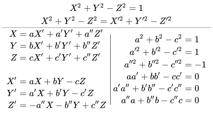
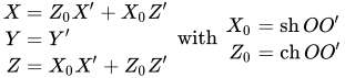
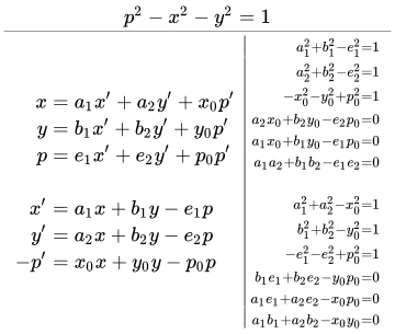
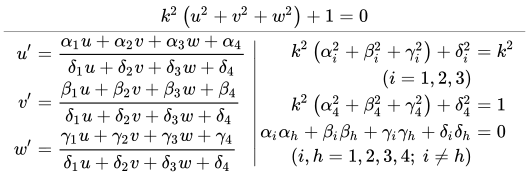
History of Lorentz transformation (edit
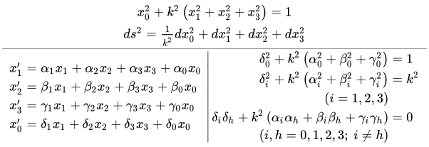
The general w:quadratic form q(x) with coefficients of a w:symmetric matrix A , the associated w:bilinear form b(x,y) , and the w:linear transformations of q(x) and b(x,y) into q(x′) and b(x′,y′) using the w:transformation matrix g , can be written as[ 1]
q
=
x
T
⋅
A
⋅
x
=
q
′
=
x
′
T
⋅
A
′
⋅
x
′
b
=
x
T
⋅
A
⋅
y
=
b
′
=
x
′
T
⋅
A
′
⋅
y
′
(
A
=
A
T
)
x
′
=
g
⋅
x
x
=
g
−
1
⋅
x
′
|
g
T
⋅
A
⋅
g
=
A
′
{\displaystyle {\begin{matrix}{\begin{aligned}q=\mathbf {x} ^{\mathrm {T} }\cdot \mathbf {A} \cdot \mathbf {x} \end{aligned}}=q'=\mathbf {x} ^{\mathrm {\prime T} }\cdot \mathbf {A} '\cdot \mathbf {x} '\\b=\mathbf {x} ^{\mathrm {T} }\cdot \mathbf {A} \cdot \mathbf {y} =b'=\mathbf {x} ^{\mathrm {\prime T} }\cdot \mathbf {A} '\cdot \mathbf {y} '\\\left(\mathbf {A} =\mathbf {A} ^{\rm {T}}\right)\\\hline \left.{\begin{aligned}\mathbf {x} '&=\mathbf {g} \cdot \mathbf {x} \\\mathbf {x} &=\mathbf {g} ^{-1}\cdot \mathbf {x} '\end{aligned}}\quad \right|\quad \mathbf {g} ^{\rm {T}}\cdot \mathbf {A} \cdot \mathbf {g} =\mathbf {A} '\end{matrix}}}
(Q1
The case n=1 is the w:binary quadratic form introduced by Lagrange (1773) and Gauss (1798/1801) , n=2 is the ternary quadratic form introduced by Gauss (1798/1801) , n=3 is the quaternary quadratic form etc.
The Lorentz interval is the invariant relation between axes and conjugate diameters of hyperbolas, illustrating Lorentz transformations between two inertial frames.
The general Lorentz transformation follows from (Q1 A =A′ =diag(-1,1,...,1) and det g =±1. It forms an w:indefinite orthogonal group called the w:Lorentz group O(1,n), while the case det g =+1 forms the restricted w:Lorentz group SO(1,n). The quadratic form q(x) becomes the w:Lorentz interval in terms of an w:indefinite quadratic form of w:Minkowski space (being a special case of w:pseudo-Euclidean space ), and the associated bilinear form b(x) becomes the w:Minkowski inner product :[ 2] [ 3]
−
x
0
2
+
⋯
+
x
n
2
=
−
x
0
′
2
+
⋯
+
x
n
′
2
−
x
0
y
0
+
⋯
+
x
n
y
n
=
−
x
0
′
y
0
′
+
⋯
+
x
n
′
y
n
′
x
′
=
g
⋅
x
↓
x
0
′
=
x
0
g
00
+
x
1
g
01
+
⋯
+
x
n
g
0
n
x
1
′
=
x
0
g
10
+
x
1
g
11
+
⋯
+
x
n
g
1
n
…
x
n
′
=
x
0
g
n
0
+
x
1
g
n
1
+
⋯
+
x
n
g
n
n
x
=
g
−
1
⋅
x
′
↓
x
0
=
x
0
′
g
00
−
x
1
′
g
10
−
⋯
−
x
n
′
g
n
0
x
1
=
−
x
0
′
g
01
+
x
1
′
g
11
+
⋯
+
x
n
′
g
n
1
…
x
n
=
−
x
0
′
g
0
n
+
x
1
′
g
1
n
+
⋯
+
x
n
′
g
n
n
|
A
⋅
g
T
⋅
A
=
g
−
1
g
T
⋅
A
⋅
g
=
A
g
⋅
A
⋅
g
T
=
A
∑
i
=
1
n
g
i
j
g
i
k
−
g
0
j
g
0
k
=
{
−
1
(
j
=
k
=
0
)
1
(
j
=
k
>
0
)
0
(
j
≠
k
)
∑
j
=
1
n
g
i
j
g
k
j
−
g
i
0
g
k
0
=
{
−
1
(
i
=
k
=
0
)
1
(
i
=
k
>
0
)
0
(
i
≠
k
)
{\displaystyle \scriptstyle {\begin{matrix}{\begin{aligned}-x_{0}^{2}+\cdots +x_{n}^{2}&=-x_{0}^{\prime 2}+\dots +x_{n}^{\prime 2}\\-x_{0}y_{0}+\cdots +x_{n}y_{n}&=-x_{0}^{\prime }y_{0}^{\prime }+\cdots +x_{n}^{\prime }y_{n}^{\prime }\end{aligned}}\\\hline \left.{\begin{matrix}\mathbf {x} '=\mathbf {g} \cdot \mathbf {x} \\\downarrow \\{\begin{aligned}x_{0}^{\prime }&=x_{0}g_{00}+x_{1}g_{01}+\dots +x_{n}g_{0n}\\x_{1}^{\prime }&=x_{0}g_{10}+x_{1}g_{11}+\dots +x_{n}g_{1n}\\&\dots \\x_{n}^{\prime }&=x_{0}g_{n0}+x_{1}g_{n1}+\dots +x_{n}g_{nn}\end{aligned}}\\\\\mathbf {x} =\mathbf {g} ^{-1}\cdot \mathbf {x} '\\\downarrow \\{\begin{aligned}x_{0}&=x_{0}^{\prime }g_{00}-x_{1}^{\prime }g_{10}-\dots -x_{n}^{\prime }g_{n0}\\x_{1}&=-x_{0}^{\prime }g_{01}+x_{1}^{\prime }g_{11}+\dots +x_{n}^{\prime }g_{n1}\\&\dots \\x_{n}&=-x_{0}^{\prime }g_{0n}+x_{1}^{\prime }g_{1n}+\dots +x_{n}^{\prime }g_{nn}\end{aligned}}\end{matrix}}\right|{\begin{matrix}{\begin{aligned}\mathbf {A} \cdot \mathbf {g} ^{\mathrm {T} }\cdot \mathbf {A} &=\mathbf {g} ^{-1}\\\mathbf {g} ^{\rm {T}}\cdot \mathbf {A} \cdot \mathbf {g} &=\mathbf {A} \\\mathbf {g} \cdot \mathbf {A} \cdot \mathbf {g} ^{\mathrm {T} }&=\mathbf {A} \\\\\end{aligned}}\\{\begin{aligned}\sum _{i=1}^{n}g_{ij}g_{ik}-g_{0j}g_{0k}&=\left\{{\begin{aligned}-1\quad &(j=k=0)\\1\quad &(j=k>0)\\0\quad &(j\neq k)\end{aligned}}\right.\\\sum _{j=1}^{n}g_{ij}g_{kj}-g_{i0}g_{k0}&=\left\{{\begin{aligned}-1\quad &(i=k=0)\\1\quad &(i=k>0)\\0\quad &(i\neq k)\end{aligned}}\right.\end{aligned}}\end{matrix}}\end{matrix}}}
(1a
The invariance of the Lorentz interval with n =1 between axes and w:conjugate diameters of hyperbolas was known for a long time since Apollonius (ca. 200 BC) . Lorentz transformations (1a Gauss (1818) , Jacobi (1827, 1833) , Lebesgue (1837) , Bour (1856) , Somov (1863) , Hill (1882) in order to simplify computations of w:elliptic functions and integrals.[ 4] [ 5] Chasles (1829) and Weddle (1847) to describe relations on hyperboloids, as well as by Poincaré (1881) , Cox (1881-91) , Picard (1882, 1884) , Killing (1885, 1893) , Gérard (1892) , Hausdorff (1899) , Woods (1901, 1903) , Liebmann (1904/05) to describe w:hyperbolic motions (i.e. rigid motions in the w:hyperbolic plane or w:hyperbolic space ), which were expressed in terms of Weierstrass coordinates of the w:hyperboloid model satisfying the relation
−
x
0
2
+
⋯
+
x
n
2
=
−
1
{\displaystyle -x_{0}^{2}+\cdots +x_{n}^{2}=-1}
w:Cayley–Klein metric of w:projective geometry using the "absolute" form
−
x
0
2
+
⋯
+
x
n
2
=
0
{\displaystyle -x_{0}^{2}+\cdots +x_{n}^{2}=0}
Klein (1871-73) .[ M 1] [ 6] [ 7] w:infinitesimal transformations related to the w:Lie algebra of the group of hyperbolic motions were given in terms of Weierstrass coordinates
−
x
0
2
+
⋯
+
x
n
2
=
−
1
{\displaystyle -x_{0}^{2}+\cdots +x_{n}^{2}=-1}
Killing (1888-1897) .
If
x
i
,
x
i
′
{\displaystyle x_{i},\ x_{i}^{\prime }}
1a w:homogeneous coordinates , then the corresponding inhomogenous coordinates
u
s
,
u
s
′
{\displaystyle u_{s},\ u_{s}^{\prime }}
x
s
x
0
=
u
s
,
x
s
′
x
0
′
=
u
s
′
(
s
=
1
,
2
…
n
)
{\displaystyle {\frac {x_{s}}{x_{0}}}=u_{s},\ {\frac {x_{s}^{\prime }}{x_{0}^{\prime }}}=u_{s}^{\prime }\ (s=1,2\dots n)}
defined by
u
1
2
+
u
2
2
+
⋯
+
u
n
2
≤
1
{\displaystyle u_{1}^{2}+u_{2}^{2}+\dots +u_{n}^{2}\leq 1}
w:homography inside the w:unit hypersphere , which w:John Lighton Synge called "the most general formula for the composition of velocities" in terms of special relativity[ 8] g stays the same as in (1a
u
s
′
=
g
s
0
+
g
s
1
u
1
+
⋯
+
g
s
n
u
n
g
00
+
g
01
u
1
+
⋯
+
g
0
n
u
n
u
s
=
−
g
0
s
+
g
1
s
u
1
′
+
⋯
+
g
n
s
u
n
′
g
00
−
g
10
u
1
′
−
⋯
−
g
n
0
u
n
′
|
∑
i
=
1
n
g
i
j
g
i
k
−
g
0
j
g
0
k
=
{
−
1
(
j
=
k
=
0
)
1
(
j
=
k
>
0
)
0
(
j
≠
k
)
∑
j
=
1
n
g
i
j
g
k
j
−
g
i
0
g
k
0
=
{
−
1
(
i
=
k
=
0
)
1
(
i
=
k
>
0
)
0
(
i
≠
k
)
{\displaystyle \scriptstyle {\begin{aligned}u_{s}^{\prime }&={\frac {g_{s0}+g_{s1}u_{1}+\dots +g_{sn}u_{n}}{g_{00}+g_{01}u_{1}+\dots +g_{0n}u_{n}}}\\\\u_{s}&={\frac {-g_{0s}+g_{1s}u_{1}^{\prime }+\dots +g_{ns}u_{n}^{\prime }}{g_{00}-g_{10}u_{1}^{\prime }-\dots -g_{n0}u_{n}^{\prime }}}\end{aligned}}\left|{\begin{aligned}\sum _{i=1}^{n}g_{ij}g_{ik}-g_{0j}g_{0k}&=\left\{{\begin{aligned}-1\quad &(j=k=0)\\1\quad &(j=k>0)\\0\quad &(j\neq k)\end{aligned}}\right.\\\sum _{j=1}^{n}g_{ij}g_{kj}-g_{i0}g_{k0}&=\left\{{\begin{aligned}-1\quad &(i=k=0)\\1\quad &(i=k>0)\\0\quad &(i\neq k)\end{aligned}}\right.\end{aligned}}\right.}
(1b
Such Lorentz transformations for various dimensions were used by Gauss (1818) , Jacobi (1827–1833) , Lebesgue (1837) , Bour (1856) , Somov (1863) , Hill (1882) , Callandreau (1885) in order to simplify computations of elliptic functions and integrals, by Picard (1882-1884) in relation to Hermitian quadratic forms , or by Woods (1901, 1903) in terms of the w:Beltrami–Klein model of hyperbolic geometry. In addition, infinitesimal transformations in terms of the w:Lie algebra of the group of hyperbolic motions leaving invariant the unit sphere
−
1
+
u
1
′
2
+
⋯
+
u
n
′
2
=
0
{\displaystyle -1+u_{1}^{\prime 2}+\cdots +u_{n}^{\prime 2}=0}
Lie (1885-1893) and Werner (1889) and Killing (1888-1897) .
Fig. 1: Apollonius' proposition illustrated by Borelli (1661) of
A
C
¯
2
−
Q
R
¯
2
=
I
L
¯
2
−
N
O
¯
2
{\displaystyle \scriptstyle {\overline {AC}}^{2}-{\overline {QR}}^{2}={\overline {IL}}^{2}-{\overline {NO}}^{2}}
w:Apollonius of Perga (c. 240–190 BC) in his 7th book on conics defined the following well known proposition (the 7th book survived in Arabian translation, and was translated into Latin in 1661 and 1710), as follows:
In every hyperbola the difference between the squares of the axes is equal to the difference between the squares of any conjugate diameters of the section. (Latin translation 1710 by w:Edmond Halley .)[ M 3] [..] in every hyperbola the difference of the squares on any two conjugate diameters is equal to the [..] difference [..] of the squares on the axes. (English translation 1896 by w:Thomas Heath .)[ M 4] Fig. 2: La Hire's (1685) illustration of
A
B
¯
2
−
D
E
¯
2
=
N
M
¯
2
−
L
K
¯
2
{\displaystyle \scriptstyle {\overline {AB}}^{2}-{\overline {DE}}^{2}={\overline {NM}}^{2}-{\overline {LK}}^{2}}
Fig. 3: l'Hôpital's (1707) illustration of
C
S
¯
2
−
C
M
¯
2
=
C
B
¯
2
−
C
A
¯
2
{\displaystyle \scriptstyle {\overline {CS}}^{2}-{\overline {CM}}^{2}={\overline {CB}}^{2}-{\overline {CA}}^{2}}
w:Philippe de La Hire (1685) stated this proposition as follows:
I say that the difference of the squares of any two diameters conjugated to each other, AB, DE, is equal to the difference of the squares of any two other diameters conjugated to each other, NM, LK.
[ M 5] and also summarized the related propositions in the 7th book of Apollonius:
In a hyperbola, the difference of the squares of the axes is equal to the difference of the squares of any two conjugate diameters.
[ M 6] w:Guillaume de l'Hôpital (1707), using the methods of w:analytic geometry , demonstrated the same proposition:[ M 7]
The difference of the squares of any two conjugate diameters "Mm, Ss" is equal to the difference of the squares of the two axes "Aa, Bb." We are to prove that
C
S
¯
2
−
C
M
¯
2
=
C
B
¯
2
−
C
A
¯
2
{\displaystyle {\overline {CS}}^{2}-{\overline {CM}}^{2}={\overline {CB}}^{2}-{\overline {CA}}^{2}}
, or
C
M
¯
2
−
C
S
¯
2
=
C
A
¯
2
−
C
B
¯
2
{\displaystyle {\overline {CM}}^{2}-{\overline {CS}}^{2}={\overline {CA}}^{2}-{\overline {CB}}^{2}}
.
(English translation 1723 by w:Edmund Stone .)[ M 8]
Apollonius' proposition can be expressed as
−
x
0
′
2
+
x
1
′
2
=
−
x
0
2
+
x
1
2
{\displaystyle -x_{0}^{\prime 2}+x_{1}^{\prime 2}=-x_{0}^{2}+x_{1}^{2}}
in agreement with the invariance of the Lorentz interval, so that the Lorentz transformation (
1a ) "(n=1)" can be interpreted as mapping from one pair of axes of a hyperbola to a pair of conjugate diameters.
Fig. 4: Apollonius' proposition illustrated by Borelli (1661) of the equality of areas of parallelogram ABCD (of the axes) and KLMN (of the conjugated diameters). Apollonius also gave another well known proposition in his 7th book regarding ellipses as well as conjugate sections of hyperbolas (see also Del Centina & Fiocca[ 9]
In the ellipse, and in conjugate sections [the opposite branches of two conjugate hyperbolas] the parallelogram bounded by the axes is equal to the parallelogram bounded by any pair of conjugate diameters, if its angles are equal to the angles the conjugate diameters form at the centre. (English translation by Del Centina & Fiocca[ 10] w:Giovanni Alfonso Borelli and w:Abraham Ecchellensis .[ M 9] If two conjugate diameters are taken in an ellipse, or in the opposite conjugate sections; the parallelogram bounded by them is equal to the rectangle bounded by the axes, provided its angles are equal to those formed at the centre by the conjugate diameters. (English translation by Del Centina & Fiocca[ 10] w:Edmond Halley .)[ M 10] If PP', DD' be two conjugate diameters in an ellipse or in conjugate hyperbolas, and if tangents be drawn at the four extremities forming a parallelogram LL'MM', then the parallelogram LL'MM' = rect. AA'·BB'. (English translation 1896 by w:Thomas Heath .)[ M 11]
The graphical representation of Apollonius proposition in Borelli's Fig. 4 is essentially a
w:Minkowski diagram , being a graphical representation of the Lorentz transformation. If line AB is the x-axis of an inertial frame S1, then line FG is the x-axis of another inertial frames S2 which together with its parallel lines (such as KL and NM) represent
w:relativity of simultaneity . Analogously, if line CD is the time axis of another inertial frame S2, then line HI is the time axis of S2 which together with its parallel lines (such as KN and LM) represent the
w:worldlines of objects at different locations. The diagonals KE (or KM) and LE (or LN) lie on the asymptotes which form a light cone. Thus the totality of all parallelograms of equal area and conjugate diameters as constructed by Apollonius, represents the totality of all inertial frames, lines of simultaneity and worldlines within a spacetime area bounded by
−
x
0
2
+
x
1
2
=
c
o
n
s
t
{\displaystyle -x_{0}^{2}+x_{1}^{2}={\rm {const}}}
.
Fig. 5: Saint-Vincent's (1647) illustration of FGHI=OPQR, as well as BADC=KNLM. w:Grégoire de Saint-Vincent independently (1647) stated the same proposition:[ M 12]
The parallelograms whose opposite sides are tangent to two conjugate hyperbolas at the extremities of two conjugate diameters are equivalent among them.
(English translation by Del Centina & Fiocca.[ 11] Fig. 6 (identical to Fig. 2): La Hire's (1685) illustration of FGHI=OPQR. w:Philippe de La Hire (1685), who was aware of both Apollonius 7th book and Saint-Vincent's book, stated this proposition as follows:[ M 13]
If a parallelogram FGHI is circumscribed about conjugate sections NA, DL, BM, KE whose sides are parallel to two conjugate diameters ED, BA drawn through their extremities, and with similar method another parallelogram OPQR is drawn through the extremities of other two conjugate diameters, then the parallelograms FGHI, OPQR are equal.
(English translation by Del Centina & Fiocca.[ 12] and also summarized the related propositions in the 7th book of Apollonius:[ M 14]
In conjugate sections and in the ellipse, the parallelogram constructed with the axes, is equal to the parallelogram constructed with any two conjugated diameters, provided the angles are equal to those between the diameters themselves.
(English translation by Del Centina & Fiocca.[ 12]
In Saint-Vincent's Fig. 5 or La Hire's Fig. 6, parallelogram FGHI contains all coordinates related to an inertial frame S3, in particular triangles EGH, EFI (Fig. 5) or CFG, CHI (Fig. 6) contain time like intervals between events on the future and past light cones, while triangles EHI, EGF (Fig. 5) or CFI, CGH (Fig. 6) contain space like intervals between events on the negative and positive x-axis. Conversely, parallelogram OPQR contains all coordinates related to another frame S4, in particular triangles EQR, EOP (Fig. 5) or CPQ, COR (Fig. 6) contain time like intervals between events on the future and past light cones, while triangles EPR, EOQ (Fig. 5) or COP, CQR (Fig. 6) contain space like intervals between events on the negative and positive x-axis.
After the invariance of the sum of squares under linear substitutions was discussed by E:Euler (1771) , the general expressions of a w:binary quadratic form and its transformation was formulated by w:Joseph-Louis Lagrange (1773/75) as follows[ M 15]
p
y
2
+
2
q
y
z
+
r
z
2
=
P
s
2
+
2
Q
s
x
+
R
x
2
y
=
M
s
+
N
x
z
=
m
s
+
n
x
|
P
=
p
M
2
+
2
q
M
m
+
r
m
2
Q
=
p
M
N
+
q
(
M
n
+
N
m
)
+
r
m
n
R
=
p
N
2
+
2
q
N
n
+
r
n
2
↓
P
R
−
Q
2
=
(
p
r
−
q
2
)
(
M
n
−
N
m
)
2
{\displaystyle {\begin{matrix}py^{2}+2qyz+rz^{2}=Ps^{2}+2Qsx+Rx^{2}\\\hline {\begin{aligned}y&=Ms+Nx\\z&=ms+nx\end{aligned}}\left|{\begin{matrix}{\begin{aligned}P&=pM^{2}+2qMm+rm^{2}\\Q&=pMN+q(Mn+Nm)+rmn\\R&=pN^{2}+2qNn+rn^{2}\end{aligned}}\\\downarrow \\PR-Q^{2}=\left(pr-q^{2}\right)(Mn-Nm)^{2}\end{matrix}}\right.\end{matrix}}}
This is equivalent to (
Q1 )
(n=1) . The Lorentz interval
−
x
0
2
+
x
1
2
{\displaystyle -x_{0}^{2}+x_{1}^{2}}
and the Lorentz transformation (
1a )
(n=1) are a special case of the binary quadratic form by setting
(p,q,r)=(P,Q,R)=(1,0,-1) .
The theory of binary quadratic forms was considerably expanded by w:Carl Friedrich Gauss (1798, published 1801) in his w:Disquisitiones Arithmeticae . He rewrote Lagrange's formalism as follows using integer coefficients α,β,γ,δ:[ M 16]
F
=
a
x
2
+
2
b
x
y
+
c
y
2
=
(
a
,
b
,
c
)
F
′
=
a
′
x
′
2
+
2
b
′
x
′
y
′
+
c
′
y
′
2
=
(
a
′
,
b
′
,
c
′
)
x
=
α
x
′
+
β
y
′
y
=
γ
x
′
+
δ
y
′
x
′
=
δ
x
−
β
y
y
′
=
−
γ
x
+
α
y
|
a
′
=
a
α
2
+
2
b
α
γ
+
c
γ
2
b
′
=
a
α
β
+
b
(
α
δ
+
β
γ
)
+
c
γ
δ
c
′
=
a
β
2
+
2
b
β
δ
+
c
δ
2
↓
b
2
−
a
′
c
′
=
(
b
2
−
a
c
)
(
α
δ
−
β
γ
)
2
{\displaystyle {\begin{matrix}F=ax^{2}+2bxy+cy^{2}=(a,b,c)\\F'=a'x^{\prime 2}+2b'x'y'+c'y^{\prime 2}=(a',b',c')\\\hline {\begin{aligned}x&=\alpha x'+\beta y'\\y&=\gamma x'+\delta y'\\\\x'&=\delta x-\beta y\\y'&=-\gamma x+\alpha y\end{aligned}}\left|{\begin{matrix}{\begin{aligned}a'&=a\alpha ^{2}+2b\alpha \gamma +c\gamma ^{2}\\b'&=a\alpha \beta +b(\alpha \delta +\beta \gamma )+c\gamma \delta \\c'&=a\beta ^{2}+2b\beta \delta +c\delta ^{2}\end{aligned}}\\\downarrow \\b^{2}-a'c'=\left(b^{2}-ac\right)(\alpha \delta -\beta \gamma )^{2}\end{matrix}}\right.\end{matrix}}}
which is equivalent to (Q1 (n=1) . As pointed out by Gauss, F and F′ are called "proper equivalent" if αδ-βγ=1, so that F is contained in F′ as well as F′ is contained in F . In addition, if another form F″ is contained by the same procedure in F′ it is also contained in F and so forth.[ M 17]
The Lorentz interval
−
x
0
2
+
x
1
2
{\displaystyle -x_{0}^{2}+x_{1}^{2}}
and the Lorentz transformation (
1a )
(n=1) are a special case of the binary quadratic form by setting
(a,b,c)=(a',b',c')=(1,0,-1) .
Gauss (1798/1801)[ M 18]
f
=
a
x
2
+
a
′
x
′
2
+
a
″
x
′
′
2
+
2
b
x
′
x
″
+
2
b
′
x
x
″
+
2
b
″
x
x
′
=
(
a
,
a
′
,
a
″
b
,
b
′
,
b
″
)
g
=
m
y
2
+
m
′
y
′
2
+
m
″
y
′
′
2
+
2
n
y
′
y
″
+
2
n
′
y
y
″
+
2
n
″
y
y
′
=
(
m
,
m
′
,
m
″
n
,
n
′
,
n
″
)
x
=
α
y
+
β
y
′
+
γ
y
″
x
′
=
α
′
y
+
β
′
y
′
+
γ
′
y
″
x
″
=
α
″
y
+
β
″
y
′
+
γ
″
y
″
{\displaystyle {\begin{matrix}f=ax^{2}+a'x^{\prime 2}+a''x^{\prime \prime 2}+2bx'x''+2b'xx''+2b''xx'=\left({\begin{matrix}a,&a',&a''\\b,&b',&b''\end{matrix}}\right)\\g=my^{2}+m'y^{\prime 2}+m''y^{\prime \prime 2}+2ny'y''+2n'yy''+2n''yy'=\left({\begin{matrix}m,&m',&m''\\n,&n',&n''\end{matrix}}\right)\\\hline {\begin{aligned}x&=\alpha y+\beta y'+\gamma y''\\x'&=\alpha 'y+\beta 'y'+\gamma 'y''\\x''&=\alpha ''y+\beta ''y'+\gamma ''y''\end{aligned}}\end{matrix}}}
which is equivalent to (Q1 (n=2) . Gauss called these forms definite when they have the same sign such as x2 +y2 +z2 , or indefinite in the case of different signs such as x2 +y2 -z2 . While discussing the classification of ternary quadratic forms, Gauss (1801) presented twenty special cases, among them these six variants:[ M 19]
(
a
,
a
′
,
a
″
b
,
b
′
,
b
″
)
⇒
(
1
,
−
1
,
1
0
,
0
,
0
)
,
(
−
1
,
1
,
1
0
,
0
,
0
)
,
(
1
,
1
,
−
1
0
,
0
,
0
)
,
(
1
,
−
1
,
−
1
0
,
0
,
0
)
,
(
−
1
,
1
,
−
1
0
,
0
,
0
)
,
(
−
1
,
−
1
,
1
0
,
0
,
0
)
{\displaystyle \left({\begin{matrix}a,&a',&a''\\b,&b',&b''\end{matrix}}\right)\Rightarrow {\begin{matrix}\left({\begin{matrix}1,&-1,&1\\0,&0,&0\end{matrix}}\right),\ \left({\begin{matrix}-1,&1,&1\\0,&0,&0\end{matrix}}\right),\ \left({\begin{matrix}1,&1,&-1\\0,&0,&0\end{matrix}}\right),\\\left({\begin{matrix}1,&-1,&-1\\0,&0,&0\end{matrix}}\right),\ \left({\begin{matrix}-1,&1,&-1\\0,&0,&0\end{matrix}}\right),\ \left({\begin{matrix}-1,&-1,&1\\0,&0,&0\end{matrix}}\right)\end{matrix}}}
These are all six types of Lorentz interval in 2+1 dimensions that can be produced as special cases of a ternary quadratic form. In general: The Lorentz interval
x
2
+
x
′
2
−
x
′
′
2
{\displaystyle x^{2}+x^{\prime 2}-x^{\prime \prime 2}}
1a (n=2) is an indefinite ternary quadratic form, which follows from the general ternary form by setting:
(
a
,
a
′
,
a
″
b
,
b
′
,
b
″
)
=
(
m
,
m
′
,
m
″
n
,
n
′
,
n
″
)
=
(
1
,
1
,
−
1
0
,
0
,
0
)
{\displaystyle \left({\begin{matrix}a,&a',&a''\\b,&b',&b''\end{matrix}}\right)=\left({\begin{matrix}m,&m',&m''\\n,&n',&n''\end{matrix}}\right)=\left({\begin{matrix}1,&1,&-1\\0,&0,&0\end{matrix}}\right)}
Gauss (1818) discussed planetary motions together with formulating w:elliptic functions . In order to simplify the integration, he transformed the expression
(
A
A
+
B
B
+
C
C
)
t
t
+
a
a
(
t
cos
E
)
2
+
b
b
(
t
sin
E
)
2
−
2
a
A
t
⋅
t
cos
E
−
2
b
B
t
⋅
t
sin
E
{\displaystyle (AA+BB+CC)tt+aa(t\cos E)^{2}+bb(t\sin E)^{2}-2aAt\cdot t\cos E-2bBt\cdot t\sin E}
into
G
+
G
′
cos
T
2
+
G
″
sin
T
2
{\displaystyle G+G'\cos T^{2}+G''\sin T^{2}}
in which the w:eccentric anomaly E is connected to the new variable T by the following transformation including an arbitrary constant k , which Gauss then rewrote by setting k =1:[ M 20]
(
α
+
α
′
cos
T
+
α
″
sin
T
)
2
+
(
β
+
β
′
cos
T
+
β
″
sin
T
)
2
−
(
γ
+
γ
′
cos
T
+
γ
″
sin
T
)
2
=
0
k
(
cos
2
T
+
sin
2
T
−
1
)
=
0
cos
E
=
α
+
α
′
cos
T
+
α
″
sin
T
γ
+
γ
′
cos
T
+
γ
″
sin
T
sin
E
=
β
+
β
′
cos
T
+
β
″
sin
T
γ
+
γ
′
cos
T
+
γ
″
sin
T
|
−
α
α
−
β
β
+
γ
γ
=
k
α
α
−
α
′
α
′
−
α
″
α
″
=
−
k
−
α
′
α
′
−
β
′
β
′
+
γ
′
γ
′
=
−
k
β
β
−
β
′
β
′
−
β
″
β
″
=
−
k
−
α
″
α
″
−
β
″
β
″
+
γ
″
γ
″
=
−
k
γ
γ
−
γ
′
γ
′
−
γ
″
γ
″
=
+
k
−
α
′
α
″
−
β
′
β
″
+
γ
′
γ
″
=
0
β
γ
−
β
′
γ
′
−
β
″
γ
″
=
0
−
α
″
α
−
β
″
β
+
γ
″
γ
=
0
γ
α
−
γ
′
α
′
−
γ
″
α
″
=
0
−
α
α
′
−
β
β
′
+
γ
γ
′
=
0
α
β
−
α
′
β
′
−
α
″
β
″
=
0
k
=
1
t
cos
E
=
α
+
α
′
cos
T
+
α
″
sin
T
t
sin
E
=
β
+
β
′
cos
T
+
β
″
sin
T
t
=
γ
+
γ
′
cos
T
+
γ
″
sin
T
|
−
α
α
−
β
β
+
γ
γ
=
1
−
α
′
α
′
−
β
′
β
′
+
γ
′
γ
′
=
−
1
−
α
″
α
″
−
β
″
β
″
+
γ
″
γ
″
=
−
1
−
α
′
α
″
−
β
′
β
″
+
γ
′
γ
″
=
0
−
α
″
α
−
β
″
β
+
γ
″
γ
=
0
−
α
α
′
−
β
β
′
+
γ
γ
′
=
0
{\displaystyle {\begin{matrix}{\scriptstyle \left(\alpha +\alpha '\cos T+\alpha ''\sin T\right)^{2}+\left(\beta +\beta '\cos T+\beta ''\sin T\right)^{2}-\left(\gamma +\gamma '\cos T+\gamma ''\sin T\right)^{2}}=0\\k\left(\cos ^{2}T+\sin ^{2}T-1\right)=0\\\hline {\begin{aligned}\cos E&={\frac {\alpha +\alpha '\cos T+\alpha ''\sin T}{\gamma +\gamma '\cos T+\gamma ''\sin T}}\\\sin E&={\frac {\beta +\beta '\cos T+\beta ''\sin T}{\gamma +\gamma '\cos T+\gamma ''\sin T}}\end{aligned}}\left|{\scriptstyle {\begin{aligned}-\alpha \alpha -\beta \beta +\gamma \gamma &=k&\alpha \alpha -\alpha '\alpha '-\alpha ''\alpha ''&=-k\\-\alpha '\alpha '-\beta '\beta '+\gamma '\gamma '&=-k&\beta \beta -\beta '\beta '-\beta ''\beta ''&=-k\\-\alpha ''\alpha ''-\beta ''\beta ''+\gamma ''\gamma ''&=-k&\gamma \gamma -\gamma '\gamma '-\gamma ''\gamma ''&=+k\\-\alpha '\alpha ''-\beta '\beta ''+\gamma '\gamma ''&=0&\beta \gamma -\beta '\gamma '-\beta ''\gamma ''&=0\\-\alpha ''\alpha -\beta ''\beta +\gamma ''\gamma &=0&\gamma \alpha -\gamma '\alpha '-\gamma ''\alpha ''&=0\\-\alpha \alpha '-\beta \beta '+\gamma \gamma '&=0&\alpha \beta -\alpha '\beta '-\alpha ''\beta ''&=0\end{aligned}}}\right.\\\hline k=1\\{\begin{aligned}t\cos E&=\alpha +\alpha '\cos T+\alpha ''\sin T\\t\sin E&=\beta +\beta '\cos T+\beta ''\sin T\\t&=\gamma +\gamma '\cos T+\gamma ''\sin T\end{aligned}}\left|{\scriptstyle {\begin{aligned}-\alpha \alpha -\beta \beta +\gamma \gamma &=1\\-\alpha '\alpha '-\beta '\beta '+\gamma '\gamma '&=-1\\-\alpha ''\alpha ''-\beta ''\beta ''+\gamma ''\gamma ''&=-1\\-\alpha '\alpha ''-\beta '\beta ''+\gamma '\gamma ''&=0\\-\alpha ''\alpha -\beta ''\beta +\gamma ''\gamma &=0\\-\alpha \alpha '-\beta \beta '+\gamma \gamma '&=0\end{aligned}}}\right.\end{matrix}}}
The coefficients α,β,γ,... of Gauss' case k =1 are equivalent to the coefficient system in Lorentz transformations (1a 1b (n=2) .
Further setting
[
cos
T
,
sin
T
,
cos
E
,
sin
E
]
=
[
u
1
,
u
2
,
u
1
′
,
u
2
′
]
{\displaystyle [\cos T,\sin T,\cos E,\sin E]=\left[u_{1},\ u_{2},\ u_{1}^{\prime },\ u_{2}^{\prime }\right]}
, Gauss' transformation becomes Lorentz transformation (
1b )
(n=2) .
Subsequently, he showed that these relations can be reformulated using three variables x,y,z and u,u′,u″ , so that
a
a
x
x
+
b
b
y
y
+
(
A
A
+
B
B
+
C
C
)
z
z
−
2
a
A
x
z
−
2
b
B
y
z
{\displaystyle aaxx+bbyy+(AA+BB+CC)zz-2aAxz-2bByz}
can be transformed into
G
u
u
+
G
′
u
′
u
′
+
G
″
u
″
u
″
{\displaystyle Guu+G'u'u'+G''u''u''}
in which x,y,z and u,u′,u″ are related by the transformation:[ M 21]
x
=
α
u
+
α
′
u
′
+
α
″
u
″
y
=
β
u
+
β
′
u
′
+
β
″
u
″
z
=
γ
u
+
γ
′
u
′
+
γ
″
u
″
u
=
−
α
x
−
β
y
+
γ
z
u
′
=
α
′
x
+
β
′
y
−
γ
′
z
u
″
=
α
″
x
+
β
″
y
−
γ
″
z
|
−
α
α
−
β
β
+
γ
γ
=
1
−
α
′
α
′
−
β
′
β
′
+
γ
′
γ
′
=
−
1
−
α
″
α
″
−
β
″
β
″
+
γ
″
γ
″
=
−
1
−
α
′
α
″
−
β
′
β
″
+
γ
′
γ
″
=
0
−
α
″
α
−
β
″
β
+
γ
″
γ
=
0
−
α
α
′
−
β
β
′
+
γ
γ
′
=
0
{\displaystyle {\begin{aligned}x&=\alpha u+\alpha 'u'+\alpha ''u''\\y&=\beta u+\beta 'u'+\beta ''u''\\z&=\gamma u+\gamma 'u'+\gamma ''u''\\\\u&=-\alpha x-\beta y+\gamma z\\u'&=\alpha 'x+\beta 'y-\gamma 'z\\u''&=\alpha ''x+\beta ''y-\gamma ''z\end{aligned}}\left|{\scriptstyle {\begin{aligned}-\alpha \alpha -\beta \beta +\gamma \gamma &=1\\-\alpha '\alpha '-\beta '\beta '+\gamma '\gamma '&=-1\\-\alpha ''\alpha ''-\beta ''\beta ''+\gamma ''\gamma ''&=-1\\-\alpha '\alpha ''-\beta '\beta ''+\gamma '\gamma ''&=0\\-\alpha ''\alpha -\beta ''\beta +\gamma ''\gamma &=0\\-\alpha \alpha '-\beta \beta '+\gamma \gamma '&=0\end{aligned}}}\right.}
This is equivalent to Lorentz transformation (
1a )
(n=2) satisfying
x
2
+
y
2
−
z
2
=
u
′
2
+
u
′
′
2
−
u
2
{\displaystyle x^{2}+y^{2}-z^{2}=u^{\prime 2}+u^{\prime \prime 2}-u^{2}}
, and can be related to Gauss' previous equations in terms of homogeneous coordinates
[
cos
T
,
sin
T
,
cos
E
,
sin
E
]
=
[
x
z
,
y
z
,
u
′
u
,
u
″
u
]
{\displaystyle \left[\cos T,\sin T,\cos E,\sin E\right]=\left[{\tfrac {x}{z}},\ {\tfrac {y}{z}},\ {\tfrac {u'}{u}},\ {\tfrac {u''}{u}}\right]}
.
Following Gauss (1818) , w:Carl Gustav Jacob Jacobi extended Gauss' transformation in 1827:[ M 22]
cos
P
2
+
sin
P
2
cos
ϑ
2
+
sin
P
2
sin
ϑ
2
=
1
k
(
cos
ψ
2
+
sin
ψ
2
cos
φ
2
+
sin
ψ
2
sin
φ
2
−
1
)
=
0
(
1
)
cos
P
=
α
+
α
′
cos
ψ
+
α
″
sin
ψ
cos
φ
+
α
‴
sin
ψ
sin
φ
δ
+
δ
′
cos
ψ
+
δ
″
sin
ψ
cos
φ
+
δ
‴
sin
ψ
sin
φ
sin
P
cos
ϑ
=
β
+
β
′
cos
ψ
+
β
″
sin
ψ
cos
φ
+
β
‴
sin
ψ
sin
φ
δ
+
δ
′
cos
ψ
+
δ
″
sin
ψ
cos
φ
+
δ
‴
sin
ψ
sin
φ
sin
P
sin
ϑ
=
γ
+
β
′
cos
ψ
+
γ
″
sin
ψ
cos
φ
+
γ
‴
sin
ψ
sin
φ
δ
+
δ
′
cos
ψ
+
δ
″
sin
ψ
cos
φ
+
δ
‴
sin
ψ
sin
φ
cos
ψ
=
−
δ
′
+
α
′
cos
P
+
β
′
sin
P
cos
ϑ
+
γ
′
sin
P
sin
ϑ
δ
−
α
cos
P
−
β
sin
P
cos
ϑ
−
γ
sin
P
sin
ϑ
sin
ψ
cos
φ
=
−
δ
″
+
α
″
cos
P
+
β
″
sin
P
cos
ϑ
+
γ
″
sin
P
sin
ϑ
δ
−
α
cos
P
−
β
sin
P
cos
ϑ
−
γ
sin
P
sin
ϑ
sin
ψ
sin
φ
=
−
δ
‴
+
α
‴
cos
P
+
β
‴
sin
P
cos
ϑ
+
γ
‴
sin
P
sin
ϑ
δ
−
α
cos
P
−
β
sin
P
cos
ϑ
−
γ
sin
P
sin
ϑ
(
2
)
α
μ
+
β
x
+
γ
y
+
δ
z
=
m
α
′
μ
+
β
′
x
+
γ
′
y
+
δ
′
z
=
m
′
α
″
μ
+
β
″
x
+
γ
″
y
+
δ
″
z
=
m
″
α
‴
μ
+
β
‴
x
+
γ
‴
y
+
δ
‴
z
=
m
‴
A
m
+
A
′
m
′
+
A
″
m
″
+
A
‴
m
‴
=
μ
B
m
+
B
′
m
′
+
B
″
m
″
+
B
‴
m
‴
=
x
C
m
+
C
′
m
′
+
C
″
m
″
+
C
‴
m
‴
=
y
D
m
+
D
′
m
′
+
D
″
m
″
+
D
‴
m
‴
=
z
α
=
−
k
A
,
β
=
−
k
B
,
γ
=
−
k
C
,
δ
=
k
D
,
α
′
=
k
A
′
,
β
′
=
k
B
′
,
γ
′
=
k
C
′
,
δ
′
=
−
k
D
′
,
α
″
=
k
A
″
,
β
″
=
k
B
″
,
γ
″
=
k
C
″
,
δ
″
=
−
k
D
″
,
α
‴
=
k
A
‴
,
β
‴
=
k
B
‴
,
γ
‴
=
k
C
‴
,
δ
‴
=
−
k
D
‴
,
|
α
α
+
β
β
+
γ
γ
−
δ
δ
=
−
k
α
′
α
′
+
β
′
β
′
+
γ
′
γ
′
−
δ
′
δ
′
=
k
α
″
α
″
+
β
″
β
″
+
γ
″
γ
″
−
δ
″
δ
″
=
k
α
‴
α
‴
+
β
‴
β
‴
+
γ
‴
γ
‴
−
δ
‴
δ
‴
=
k
α
α
′
+
β
β
′
+
γ
γ
′
−
δ
δ
′
=
0
α
α
″
+
β
β
″
+
γ
γ
″
−
δ
δ
″
=
0
α
α
‴
+
β
β
‴
+
γ
γ
‴
−
δ
δ
‴
=
0
α
″
α
‴
+
β
″
β
‴
+
γ
″
γ
‴
−
δ
″
δ
‴
=
0
α
‴
α
′
+
β
‴
β
′
+
γ
‴
γ
′
−
δ
‴
δ
′
=
0
α
′
α
″
+
β
′
β
″
+
γ
′
γ
″
−
δ
′
δ
″
=
0
−
α
α
+
α
′
α
′
+
α
″
α
″
+
α
‴
α
‴
=
k
−
β
β
+
β
′
β
′
+
β
″
β
″
+
β
‴
β
‴
=
k
−
γ
γ
+
γ
′
γ
′
+
γ
″
γ
″
+
γ
‴
γ
‴
=
k
−
δ
δ
+
δ
′
δ
′
+
δ
″
δ
″
+
δ
‴
δ
‴
=
−
k
−
α
β
+
α
′
β
′
+
α
″
β
″
+
α
‴
β
‴
=
0
−
α
γ
+
α
′
γ
′
+
α
″
γ
″
+
α
‴
γ
‴
=
0
−
α
δ
+
α
′
δ
′
+
α
″
δ
″
+
α
‴
δ
‴
=
0
−
β
γ
+
β
′
γ
′
+
β
″
γ
″
+
β
‴
γ
‴
=
0
−
γ
δ
+
γ
′
δ
′
+
γ
″
δ
″
+
γ
‴
δ
‴
=
0
−
δ
β
+
δ
′
β
′
+
δ
″
β
″
+
δ
‴
β
‴
=
0
{\displaystyle {\scriptstyle {\begin{matrix}\cos P^{2}+\sin P^{2}\cos \vartheta ^{2}+\sin P^{2}\sin \vartheta ^{2}=1\\k\left(\cos \psi ^{2}+\sin \psi ^{2}\cos \varphi ^{2}+\sin \psi ^{2}\sin \varphi ^{2}-1\right)=0\\\hline {\left.{\begin{matrix}\mathbf {(1)} {\begin{aligned}\cos P&={\frac {\alpha +\alpha '\cos \psi +\alpha ''\sin \psi \cos \varphi +\alpha '''\sin \psi \sin \varphi }{\delta +\delta '\cos \psi +\delta ''\sin \psi \cos \varphi +\delta '''\sin \psi \sin \varphi }}\\\sin P\cos \vartheta &={\frac {\beta +\beta '\cos \psi +\beta ''\sin \psi \cos \varphi +\beta '''\sin \psi \sin \varphi }{\delta +\delta '\cos \psi +\delta ''\sin \psi \cos \varphi +\delta '''\sin \psi \sin \varphi }}\\\sin P\sin \vartheta &={\frac {\gamma +\beta '\cos \psi +\gamma ''\sin \psi \cos \varphi +\gamma '''\sin \psi \sin \varphi }{\delta +\delta '\cos \psi +\delta ''\sin \psi \cos \varphi +\delta '''\sin \psi \sin \varphi }}\\\\\cos \psi &={\frac {-\delta '+\alpha '\cos P+\beta '\sin P\cos \vartheta +\gamma '\sin P\sin \vartheta }{\delta -\alpha \cos P-\beta \sin P\cos \vartheta -\gamma \sin P\sin \vartheta }}\\\sin \psi \cos \varphi &={\frac {-\delta ''+\alpha ''\cos P+\beta ''\sin P\cos \vartheta +\gamma ''\sin P\sin \vartheta }{\delta -\alpha \cos P-\beta \sin P\cos \vartheta -\gamma \sin P\sin \vartheta }}\\\sin \psi \sin \varphi &={\frac {-\delta '''+\alpha '''\cos P+\beta '''\sin P\cos \vartheta +\gamma '''\sin P\sin \vartheta }{\delta -\alpha \cos P-\beta \sin P\cos \vartheta -\gamma \sin P\sin \vartheta }}\end{aligned}}\\\\\hline \mathbf {(2)} {\begin{aligned}\alpha \mu +\beta x+\gamma y+\delta z&=m\\\alpha '\mu +\beta 'x+\gamma 'y+\delta 'z&=m'\\\alpha ''\mu +\beta ''x+\gamma ''y+\delta ''z&=m''\\\alpha '''\mu +\beta '''x+\gamma '''y+\delta '''z&=m'''\\\\Am+A'm'+A''m''+A'''m'''&=\mu \\Bm+B'm'+B''m''+B'''m'''&=x\\Cm+C'm'+C''m''+C'''m'''&=y\\Dm+D'm'+D''m''+D'''m'''&=z\\\\\end{aligned}}\\{\begin{aligned}\alpha &=-kA,&\beta &=-kB,&\gamma &=-kC,&\delta &=kD,\\\alpha '&=kA',&\beta '&=kB',&\gamma '&=kC',&\delta '&=-kD',\\\alpha ''&=kA'',&\beta ''&=kB'',&\gamma ''&=kC'',&\delta ''&=-kD'',\\\alpha '''&=kA''',&\beta '''&=kB''',&\gamma '''&=kC''',&\delta '''&=-kD''',\end{aligned}}\end{matrix}}\right|{\begin{matrix}{\begin{aligned}\alpha \alpha +\beta \beta +\gamma \gamma -\delta \delta &=-k\\\alpha '\alpha '+\beta '\beta '+\gamma '\gamma '-\delta '\delta '&=k\\\alpha ''\alpha ''+\beta ''\beta ''+\gamma ''\gamma ''-\delta ''\delta ''&=k\\\alpha '''\alpha '''+\beta '''\beta '''+\gamma '''\gamma '''-\delta '''\delta '''&=k\\\alpha \alpha '+\beta \beta '+\gamma \gamma '-\delta \delta '&=0\\\alpha \alpha ''+\beta \beta ''+\gamma \gamma ''-\delta \delta ''&=0\\\alpha \alpha '''+\beta \beta '''+\gamma \gamma '''-\delta \delta '''&=0\\\alpha ''\alpha '''+\beta ''\beta '''+\gamma ''\gamma '''-\delta ''\delta '''&=0\\\alpha '''\alpha '+\beta '''\beta '+\gamma '''\gamma '-\delta '''\delta '&=0\\\alpha '\alpha ''+\beta '\beta ''+\gamma '\gamma ''-\delta '\delta ''&=0\\\\-\alpha \alpha +\alpha '\alpha '+\alpha ''\alpha ''+\alpha '''\alpha '''&=k\\-\beta \beta +\beta '\beta '+\beta ''\beta ''+\beta '''\beta '''&=k\\-\gamma \gamma +\gamma '\gamma '+\gamma ''\gamma ''+\gamma '''\gamma '''&=k\\-\delta \delta +\delta '\delta '+\delta ''\delta ''+\delta '''\delta '''&=-k\\-\alpha \beta +\alpha '\beta '+\alpha ''\beta ''+\alpha '''\beta '''&=0\\-\alpha \gamma +\alpha '\gamma '+\alpha ''\gamma ''+\alpha '''\gamma '''&=0\\-\alpha \delta +\alpha '\delta '+\alpha ''\delta ''+\alpha '''\delta '''&=0\\-\beta \gamma +\beta '\gamma '+\beta ''\gamma ''+\beta '''\gamma '''&=0\\-\gamma \delta +\gamma '\delta '+\gamma ''\delta ''+\gamma '''\delta '''&=0\\-\delta \beta +\delta '\beta '+\delta ''\beta ''+\delta '''\beta '''&=0\end{aligned}}\end{matrix}}}\end{matrix}}}}
By setting
[
cos
P
,
sin
P
cos
φ
,
sin
P
sin
φ
]
=
[
u
1
,
u
2
,
u
3
]
[
cos
ψ
,
sin
ψ
cos
ϑ
,
sin
ψ
sin
ϑ
]
=
[
u
1
′
,
u
2
′
,
u
3
′
]
{\displaystyle {\scriptstyle {\begin{aligned}\left[\cos P,\ \sin P\cos \varphi ,\ \sin P\sin \varphi \right]&=\left[u_{1},\ u_{2},\ u_{3}\right]\\{}[\cos \psi ,\ \sin \psi \cos \vartheta ,\ \sin \psi \sin \vartheta ]&=\left[u_{1}^{\prime },\ u_{2}^{\prime },\ u_{3}^{\prime }\right]\end{aligned}}}}
and
k =1 in the (1827) formulas, transformation system (1) is equivalent to Lorentz transformation (
1b )
(n=3) , and by setting
k =1 in transformation system (2) it becomes equivalent to Lorentz transformation (
1a )
(n=3) producing
m
2
+
m
′
2
+
m
′
′
2
−
m
′
′
′
2
=
μ
2
+
x
2
+
y
2
−
z
2
{\displaystyle m^{2}+m^{\prime 2}+m^{\prime \prime 2}-m^{\prime \prime \prime 2}=\mu ^{2}+x^{2}+y^{2}-z^{2}}
.
Alternatively, in two papers from 1832 Jacobi started with an ordinary orthogonal transformation, and by using an imaginary substitution he arrived at Gauss' transformation (up to a sign change):[ M 23]
x
x
+
y
y
+
z
z
=
s
s
+
s
′
s
′
+
s
″
s
″
=
0
(
1
)
x
=
α
s
+
α
′
s
′
+
α
″
s
″
y
=
β
s
+
β
′
s
′
+
β
″
s
″
z
=
γ
s
+
γ
′
s
′
+
γ
″
s
″
s
=
α
x
+
β
y
+
γ
z
s
′
=
α
′
x
+
β
′
y
+
γ
′
z
s
″
=
α
″
x
+
β
″
y
+
γ
″
z
|
α
α
+
β
β
+
γ
γ
=
1
α
α
+
α
′
α
′
+
α
″
α
″
=
1
α
′
α
′
+
β
′
β
′
+
γ
′
γ
′
=
1
β
β
+
β
′
β
′
+
β
″
β
″
=
1
α
″
α
″
+
β
″
β
″
+
γ
″
γ
″
=
1
γ
γ
+
γ
′
γ
′
+
γ
″
γ
″
=
1
α
′
α
″
+
β
′
β
″
+
γ
′
γ
″
=
0
β
γ
+
β
′
γ
′
+
β
″
γ
″
=
0
α
″
α
+
β
″
β
+
γ
″
γ
=
0
γ
α
+
γ
′
α
′
+
γ
″
α
″
=
0
α
α
′
+
β
β
′
+
γ
γ
′
=
0
α
β
+
α
′
β
′
+
α
″
β
″
=
0
[
y
x
,
z
x
,
s
′
s
,
s
″
s
]
=
[
−
i
cos
φ
,
−
i
sin
φ
,
i
cos
η
,
i
sin
η
]
[
α
′
,
α
″
,
β
,
γ
]
=
[
i
α
′
,
i
α
″
,
−
i
β
,
−
i
γ
]
(
2
)
(
α
−
α
′
cos
η
−
α
″
sin
η
)
2
=
(
β
−
β
′
cos
η
−
β
″
sin
η
)
2
+
(
γ
−
γ
′
cos
η
−
γ
″
sin
η
)
2
(
α
−
β
cos
ϕ
−
γ
sin
ϕ
)
2
=
(
α
′
−
β
′
cos
ϕ
−
γ
′
sin
ϕ
)
2
+
(
α
″
−
β
″
cos
ϕ
−
γ
″
sin
ϕ
)
2
cos
ϕ
=
β
−
β
′
cos
η
−
β
″
sin
η
α
−
α
′
cos
η
−
α
″
sin
η
,
cos
η
=
α
′
−
β
′
cos
ϕ
−
γ
′
sin
ϕ
α
−
β
cos
ϕ
−
γ
sin
ϕ
sin
ϕ
=
γ
−
γ
′
cos
η
−
γ
″
sin
η
α
−
α
′
cos
η
−
α
″
sin
η
,
sin
η
=
α
″
−
β
″
cos
ϕ
−
γ
″
sin
ϕ
α
−
β
cos
ϕ
−
γ
sin
ϕ
(
3
)
1
−
z
z
−
y
y
=
1
−
s
′
s
′
−
s
″
s
″
(
α
−
α
′
s
′
−
α
″
s
″
)
2
y
=
β
−
β
′
s
′
−
β
″
s
″
α
−
α
′
s
′
−
α
″
s
″
,
s
′
=
α
′
−
β
′
y
−
γ
′
z
α
−
β
y
−
γ
z
,
z
=
γ
−
γ
′
s
′
−
γ
″
s
″
α
−
α
′
s
′
−
α
″
s
‴
,
s
″
=
α
″
−
β
″
y
−
γ
″
z
α
−
β
y
−
γ
z
,
|
α
α
−
β
β
−
γ
γ
=
1
α
′
α
′
−
β
′
β
′
−
γ
′
γ
′
=
−
1
α
″
α
″
−
β
″
β
″
−
γ
″
γ
″
=
−
1
α
′
α
″
−
β
′
β
″
−
γ
′
γ
″
=
0
α
″
α
−
β
″
β
−
γ
″
γ
=
0
α
α
′
−
β
β
′
−
γ
γ
′
=
0
α
α
−
α
′
α
′
−
α
″
α
″
=
1
β
β
−
β
′
β
′
−
β
″
β
″
=
−
1
γ
γ
−
γ
′
γ
′
−
γ
″
γ
″
=
−
1
β
γ
−
β
′
γ
′
−
β
″
γ
″
=
0
γ
α
−
γ
′
α
′
−
γ
″
α
″
=
0
α
β
−
α
′
β
′
−
α
″
β
″
=
0
{\displaystyle {\scriptstyle {\begin{matrix}xx+yy+zz=ss+s's'+s''s''=0\\\mathbf {(1)} {\begin{aligned}x&=\alpha s+\alpha 's'+\alpha ''s''\\y&=\beta s+\beta 's'+\beta ''s''\\z&=\gamma s+\gamma 's'+\gamma ''s''\\\\s&=\alpha x+\beta y+\gamma z\\s'&=\alpha 'x+\beta 'y+\gamma 'z\\s''&=\alpha ''x+\beta ''y+\gamma ''z\end{aligned}}\left|{\begin{aligned}\alpha \alpha +\beta \beta +\gamma \gamma &=1&\alpha \alpha +\alpha '\alpha '+\alpha ''\alpha ''&=1\\\alpha '\alpha '+\beta '\beta '+\gamma '\gamma '&=1&\beta \beta +\beta '\beta '+\beta ''\beta ''&=1\\\alpha ''\alpha ''+\beta ''\beta ''+\gamma ''\gamma ''&=1&\gamma \gamma +\gamma '\gamma '+\gamma ''\gamma ''&=1\\\alpha '\alpha ''+\beta '\beta ''+\gamma '\gamma ''&=0&\beta \gamma +\beta '\gamma '+\beta ''\gamma ''&=0\\\alpha ''\alpha +\beta ''\beta +\gamma ''\gamma &=0&\gamma \alpha +\gamma '\alpha '+\gamma ''\alpha ''&=0\\\alpha \alpha '+\beta \beta '+\gamma \gamma '&=0&\alpha \beta +\alpha '\beta '+\alpha ''\beta ''&=0\end{aligned}}\right.\\\hline \left[{\frac {y}{x}},\ {\frac {z}{x}},\ {\frac {s'}{s}},\ {\frac {s''}{s}}\right]=\left[-i\cos \varphi ,\ -i\sin \varphi ,\ i\cos \eta ,\ i\sin \eta \right]\\\left[\alpha ',\ \alpha '',\ \beta ,\ \gamma \right]=\left[i\alpha ',\ i\alpha '',\ -i\beta ,\ -i\gamma \right]\\\hline {\begin{matrix}\mathbf {(2)} {\begin{matrix}\left(\alpha -\alpha '\cos \eta -\alpha ''\sin \eta \right)^{2}=\left(\beta -\beta '\cos \eta -\beta ''\sin \eta \right)^{2}+\left(\gamma -\gamma '\cos \eta -\gamma ''\sin \eta \right)^{2}\\\left(\alpha -\beta \cos \phi -\gamma \sin \phi \right)^{2}=\left(\alpha '-\beta '\cos \phi -\gamma '\sin \phi \right)^{2}+\left(\alpha ''-\beta ''\cos \phi -\gamma ''\sin \phi \right)^{2}\\\hline {\begin{aligned}\cos \phi &={\frac {\beta -\beta '\cos \eta -\beta ''\sin \eta }{\alpha -\alpha '\cos \eta -\alpha ''\sin \eta }},&\cos \eta &={\frac {\alpha '-\beta '\cos \phi -\gamma '\sin \phi }{\alpha -\beta \cos \phi -\gamma \sin \phi }}\\\sin \phi &={\frac {\gamma -\gamma '\cos \eta -\gamma ''\sin \eta }{\alpha -\alpha '\cos \eta -\alpha ''\sin \eta }},&\sin \eta &={\frac {\alpha ''-\beta ''\cos \phi -\gamma ''\sin \phi }{\alpha -\beta \cos \phi -\gamma \sin \phi }}\end{aligned}}\end{matrix}}\\\hline \\\mathbf {(3)} {\begin{matrix}1-zz-yy={\frac {1-s's'-s''s''}{\left(\alpha -\alpha 's'-\alpha ''s''\right)^{2}}}\\\hline {\begin{aligned}y&={\frac {\beta -\beta 's'-\beta ''s''}{\alpha -\alpha 's'-\alpha ''s''}},&s'&={\frac {\alpha '-\beta 'y-\gamma 'z}{\alpha -\beta y-\gamma z}},\\z&={\frac {\gamma -\gamma 's'-\gamma ''s''}{\alpha -\alpha 's'-\alpha ''s'''}},&s''&={\frac {\alpha ''-\beta ''y-\gamma ''z}{\alpha -\beta y-\gamma z}},\end{aligned}}\end{matrix}}\end{matrix}}\left|{\begin{aligned}\alpha \alpha -\beta \beta -\gamma \gamma &=1\\\alpha '\alpha '-\beta '\beta '-\gamma '\gamma '&=-1\\\alpha ''\alpha ''-\beta ''\beta ''-\gamma ''\gamma ''&=-1\\\alpha '\alpha ''-\beta '\beta ''-\gamma '\gamma ''&=0\\\alpha ''\alpha -\beta ''\beta -\gamma ''\gamma &=0\\\alpha \alpha '-\beta \beta '-\gamma \gamma '&=0\\\\\alpha \alpha -\alpha '\alpha '-\alpha ''\alpha ''&=1\\\beta \beta -\beta '\beta '-\beta ''\beta ''&=-1\\\gamma \gamma -\gamma '\gamma '-\gamma ''\gamma ''&=-1\\\beta \gamma -\beta '\gamma '-\beta ''\gamma ''&=0\\\gamma \alpha -\gamma '\alpha '-\gamma ''\alpha ''&=0\\\alpha \beta -\alpha '\beta '-\alpha ''\beta ''&=0\end{aligned}}\right.\end{matrix}}}}
By setting
[
cos
ϕ
,
sin
ϕ
,
cos
η
,
sin
η
]
=
[
u
1
,
u
2
,
u
1
′
,
u
2
′
]
{\displaystyle [\cos \phi ,\ \sin \phi ,\ \cos \eta ,\ \sin \eta ]=\left[u_{1},\ u_{2},\ u_{1}^{\prime },\ u_{2}^{\prime }\right]}
, transformation system (2) is equivalent to Lorentz transformation (
1b )
(n=2) . Also transformation system (3) is equivalent to Lorentz transformation (
1b )
(n=2) up to a sign change.
Extending his previous result, Jacobi (1833) started with Cauchy's (1829) orthogonal transformation for n dimensions, and by using an imaginary substitution he formulated Gauss' transformation (up to a sign change) in the case of n dimensions:[ M 24]
x
1
x
1
+
x
2
x
2
+
⋯
+
x
n
x
n
=
y
1
y
1
+
y
2
y
2
+
⋯
+
y
n
y
n
(
1
)
y
ϰ
=
α
1
(
ϰ
)
x
1
+
α
2
(
ϰ
)
x
2
+
⋯
+
α
n
(
ϰ
)
x
n
x
ϰ
=
α
ϰ
′
y
1
+
α
ϰ
′
′
y
2
+
⋯
+
α
ϰ
(
n
)
y
n
y
ϰ
y
n
=
α
1
(
ϰ
)
x
1
+
α
2
(
ϰ
)
x
2
+
⋯
+
α
n
(
ϰ
)
x
n
α
1
(
n
)
x
1
+
α
2
(
n
)
x
2
+
⋯
+
α
n
(
n
)
x
n
x
ϰ
x
n
=
α
ϰ
′
y
1
+
α
ϰ
′
′
y
2
+
⋯
+
α
ϰ
(
n
)
y
n
α
1
(
n
)
x
1
+
α
2
(
n
)
x
2
+
⋯
+
α
n
(
n
)
x
n
|
α
ϰ
′
α
λ
′
+
α
ϰ
′
′
α
λ
′
′
+
⋯
+
α
ϰ
(
n
)
α
λ
(
n
)
=
0
α
ϰ
′
α
ϰ
′
+
α
ϰ
′
′
α
ϰ
′
′
+
⋯
+
α
ϰ
(
n
)
α
ϰ
(
n
)
=
1
α
1
(
ϰ
)
α
1
(
λ
)
+
α
2
(
ϰ
)
α
2
(
λ
)
+
⋯
+
α
n
(
ϰ
)
α
n
(
λ
)
=
0
α
1
(
ϰ
)
α
1
(
ϰ
)
+
α
2
(
ϰ
)
α
2
(
ϰ
)
+
⋯
+
α
n
(
ϰ
)
α
n
(
ϰ
)
=
1
x
ϰ
x
n
=
−
i
ξ
ϰ
,
y
ϰ
y
n
=
i
ν
ϰ
1
−
ξ
1
ξ
1
−
ξ
2
ξ
2
−
⋯
−
ξ
n
−
1
ξ
n
−
1
=
y
n
y
n
x
n
x
n
(
1
−
ν
1
ν
1
−
ν
2
ν
2
−
⋯
−
ν
n
−
1
ν
n
−
1
)
α
n
(
ϰ
)
=
i
α
(
ϰ
)
,
α
ϰ
(
n
)
=
−
i
α
ϰ
,
α
n
(
n
)
=
α
1
−
ξ
1
ξ
1
−
ξ
2
ξ
2
−
⋯
−
ξ
n
−
1
ξ
n
−
1
=
1
−
ν
1
ν
1
−
ν
2
ν
2
−
⋯
−
ν
n
−
1
ν
n
−
1
[
α
−
α
′
ν
1
−
α
′
′
ν
2
⋯
−
α
(
n
−
1
)
ν
n
−
1
]
2
(
2
)
ν
ϰ
=
α
(
ϰ
)
−
α
1
(
ϰ
)
ξ
1
−
α
2
(
ϰ
)
ξ
2
⋯
−
α
n
−
1
(
ϰ
)
ξ
n
−
1
α
−
α
1
ξ
1
−
α
2
ξ
2
⋯
−
α
n
−
1
ξ
n
−
1
ξ
ϰ
=
α
ϰ
−
α
ϰ
′
ν
1
−
α
2
′
′
ν
2
⋯
−
α
ϰ
(
n
−
1
)
ν
n
−
1
α
−
α
′
ν
1
−
α
′
′
ν
2
⋯
−
α
(
n
−
1
)
ν
n
−
1
ξ
1
ξ
1
−
ξ
2
ξ
2
−
⋯
−
ξ
n
−
1
ξ
n
−
1
=
1
⇒
ν
1
ν
1
−
ν
2
ν
2
−
⋯
−
ν
n
−
1
ν
n
−
1
=
1
{\displaystyle {\scriptstyle {\begin{matrix}x_{1}x_{1}+x_{2}x_{2}+\dots +x_{n}x_{n}=y_{1}y_{1}+y_{2}y_{2}+\dots +y_{n}y_{n}\\\hline \mathbf {(1)\ } {\begin{aligned}y_{\varkappa }&=\alpha _{1}^{(\varkappa )}x_{1}+\alpha _{2}^{(\varkappa )}x_{2}+\dots +\alpha _{n}^{(\varkappa )}x_{n}\\x_{\varkappa }&=\alpha _{\varkappa }^{\prime }y_{1}+\alpha _{\varkappa }^{\prime \prime }y_{2}+\dots +\alpha _{\varkappa }^{(n)}y_{n}\\\\{\frac {y_{\varkappa }}{y_{n}}}&={\frac {\alpha _{1}^{(\varkappa )}x_{1}+\alpha _{2}^{(\varkappa )}x_{2}+\dots +\alpha _{n}^{(\varkappa )}x_{n}}{\alpha _{1}^{(n)}x_{1}+\alpha _{2}^{(n)}x_{2}+\dots +\alpha _{n}^{(n)}x_{n}}}\\{\frac {x_{\varkappa }}{x_{n}}}&={\frac {\alpha _{\varkappa }^{\prime }y_{1}+\alpha _{\varkappa }^{\prime \prime }y_{2}+\dots +\alpha _{\varkappa }^{(n)}y_{n}}{\alpha _{1}^{(n)}x_{1}+\alpha _{2}^{(n)}x_{2}+\dots +\alpha _{n}^{(n)}x_{n}}}\end{aligned}}\left|{\begin{aligned}\alpha _{\varkappa }^{\prime }\alpha _{\lambda }^{\prime }+\alpha _{\varkappa }^{\prime \prime }\alpha _{\lambda }^{\prime \prime }+\dots +\alpha _{\varkappa }^{(n)}\alpha _{\lambda }^{(n)}&=0\\\alpha _{\varkappa }^{\prime }\alpha _{\varkappa }^{\prime }+\alpha _{\varkappa }^{\prime \prime }\alpha _{\varkappa }^{\prime \prime }+\dots +\alpha _{\varkappa }^{(n)}\alpha _{\varkappa }^{(n)}&=1\\\\\alpha _{1}^{(\varkappa )}\alpha _{1}^{(\lambda )}+\alpha _{2}^{(\varkappa )}\alpha _{2}^{(\lambda )}+\dots +\alpha _{n}^{(\varkappa )}\alpha _{n}^{(\lambda )}&=0\\\alpha _{1}^{(\varkappa )}\alpha _{1}^{(\varkappa )}+\alpha _{2}^{(\varkappa )}\alpha _{2}^{(\varkappa )}+\dots +\alpha _{n}^{(\varkappa )}\alpha _{n}^{(\varkappa )}&=1\end{aligned}}\right.\\\hline {\frac {x_{\varkappa }}{x_{n}}}=-i\xi _{\varkappa },\ {\frac {y_{\varkappa }}{y_{n}}}=i\nu _{\varkappa }\\1-\xi _{1}\xi _{1}-\xi _{2}\xi _{2}-\dots -\xi _{n-1}\xi _{n-1}={\frac {y_{n}y_{n}}{x_{n}x_{n}}}\left(1-\nu _{1}\nu _{1}-\nu _{2}\nu _{2}-\dots -\nu _{n-1}\nu _{n-1}\right)\\\alpha _{n}^{(\varkappa )}=i\alpha ^{(\varkappa )},\ \alpha _{\varkappa }^{(n)}=-i\alpha _{\varkappa },\ \alpha _{n}^{(n)}=\alpha \\1-\xi _{1}\xi _{1}-\xi _{2}\xi _{2}-\dots -\xi _{n-1}\xi _{n-1}={\frac {1-\nu _{1}\nu _{1}-\nu _{2}\nu _{2}-\dots -\nu _{n-1}\nu _{n-1}}{\left[\alpha -\alpha ^{\prime }\nu _{1}-\alpha ^{\prime \prime }\nu _{2}\dots -\alpha ^{(n-1)}\nu _{n-1}\right]^{2}}}\\\hline \mathbf {(2)\ } {\begin{aligned}\nu _{\varkappa }&={\frac {\alpha ^{(\varkappa )}-\alpha _{1}^{(\varkappa )}\xi _{1}-\alpha _{2}^{(\varkappa )}\xi _{2}\dots -\alpha _{n-1}^{(\varkappa )}\xi _{n-1}}{\alpha -\alpha _{1}\xi _{1}-\alpha _{2}\xi _{2}\dots -\alpha _{n-1}\xi _{n-1}}}\\\\\xi _{\varkappa }&={\frac {\alpha _{\varkappa }-\alpha _{\varkappa }^{\prime }\nu _{1}-\alpha _{2}^{\prime \prime }\nu _{2}\dots -\alpha _{\varkappa }^{(n-1)}\nu _{n-1}}{\alpha -\alpha ^{\prime }\nu _{1}-\alpha ^{\prime \prime }\nu _{2}\dots -\alpha ^{(n-1)}\nu _{n-1}}}\end{aligned}}\\\hline \xi _{1}\xi _{1}-\xi _{2}\xi _{2}-\dots -\xi _{n-1}\xi _{n-1}=1\ \Rightarrow \ \nu _{1}\nu _{1}-\nu _{2}\nu _{2}-\dots -\nu _{n-1}\nu _{n-1}=1\end{matrix}}}}
Transformation system (2) is equivalent to Lorentz transformation (
1b ) up to a sign change.
He also stated the following transformation leaving invariant the Lorentz interval:[ M 25]
u
u
−
u
1
u
1
−
u
2
u
2
−
⋯
−
u
n
−
1
u
n
−
1
=
w
w
−
w
1
w
1
−
w
2
w
2
−
⋯
−
w
n
−
1
w
n
−
1
u
=
α
w
−
α
′
w
1
−
α
″
w
2
−
⋯
−
α
(
n
−
1
)
w
n
−
1
u
1
=
α
1
w
−
α
1
′
w
1
−
α
1
′
′
w
2
−
⋯
−
α
1
(
n
−
1
)
w
n
−
1
…
u
n
−
1
=
α
n
−
1
w
−
α
n
−
1
′
w
1
−
α
n
−
1
′
′
w
2
−
⋯
−
α
n
−
1
(
n
−
1
)
w
n
−
1
w
=
α
u
−
α
1
u
1
−
α
2
′
′
u
2
−
⋯
−
α
n
−
1
u
n
−
1
w
1
=
α
′
u
−
α
1
′
u
1
−
α
2
′
u
2
−
⋯
−
α
n
−
1
′
u
n
−
1
…
w
n
−
1
=
α
(
n
−
1
)
u
−
α
1
(
n
−
1
)
u
1
−
α
2
(
n
−
1
)
u
2
−
⋯
−
α
n
−
1
(
n
−
1
)
u
n
−
1
|
α
α
−
α
′
α
′
−
α
″
α
″
⋯
−
α
(
n
−
1
)
α
(
n
−
1
)
=
+
1
α
ϰ
α
ϰ
−
α
ϰ
′
α
ϰ
′
−
α
ϰ
′
′
α
ϰ
′
′
⋯
−
α
ϰ
(
n
−
1
)
α
ϰ
(
n
−
1
)
=
−
1
α
α
ϰ
−
α
′
α
ϰ
′
−
α
′
′
α
ϰ
′
′
⋯
−
α
(
n
−
1
)
α
ϰ
(
n
−
1
)
=
0
α
ϰ
α
λ
−
α
ϰ
′
α
λ
′
−
α
ϰ
′
′
α
λ
′
′
⋯
−
α
ϰ
(
n
−
1
)
α
λ
(
n
−
1
)
=
0
α
α
−
α
1
α
1
−
α
2
α
2
⋯
−
α
n
−
1
α
n
−
1
=
+
1
α
ϰ
α
ϰ
−
α
1
ϰ
α
1
ϰ
−
α
2
′
′
α
2
′
′
⋯
−
α
n
−
1
(
ϰ
)
α
n
−
1
(
ϰ
)
=
−
1
α
α
(
ϰ
)
−
α
1
α
1
(
ϰ
)
−
α
2
α
2
(
ϰ
)
⋯
−
α
n
−
1
α
n
−
1
(
ϰ
)
=
0
α
(
ϰ
)
α
(
λ
)
−
α
1
(
ϰ
)
α
1
λ
l
)
−
α
2
(
ϰ
)
α
2
(
λ
)
⋯
−
α
n
−
1
(
ϰ
)
α
n
−
1
(
λ
)
=
0
{\displaystyle {\begin{matrix}uu-u_{1}u_{1}-u_{2}u_{2}-\dots -u_{n-1}u_{n-1}=ww-w_{1}w_{1}-w_{2}w_{2}-\dots -w_{n-1}w_{n-1}\\\hline {\scriptstyle {\begin{aligned}u&=\alpha w-\alpha 'w_{1}-\alpha ''w_{2}-\dots -\alpha ^{(n-1)}w_{n-1}\\u_{1}&=\alpha _{1}w-\alpha _{1}^{\prime }w_{1}-\alpha _{1}^{\prime \prime }w_{2}-\dots -\alpha _{1}^{(n-1)}w_{n-1}\\&\dots \\u_{n-1}&=\alpha _{n-1}w-\alpha _{n-1}^{\prime }w_{1}-\alpha _{n-1}^{\prime \prime }w_{2}-\dots -\alpha _{n-1}^{(n-1)}w_{n-1}\\\\w&=\alpha u-\alpha _{1}u_{1}-\alpha _{2}^{\prime \prime }u_{2}-\dots -\alpha _{n-1}u_{n-1}\\w_{1}&=\alpha 'u-\alpha _{1}^{\prime }u_{1}-\alpha _{2}^{\prime }u_{2}-\dots -\alpha _{n-1}^{\prime }u_{n-1}\\&\dots \\w_{n-1}&=\alpha ^{(n-1)}u-\alpha _{1}^{(n-1)}u_{1}-\alpha _{2}^{(n-1)}u_{2}-\dots -\alpha _{n-1}^{(n-1)}u_{n-1}\end{aligned}}\left|{\begin{aligned}\alpha \alpha -\alpha '\alpha '-\alpha ''\alpha ''\dots -\alpha ^{(n-1)}\alpha ^{(n-1)}&=+1\\\alpha _{\varkappa }\alpha _{\varkappa }-\alpha _{\varkappa }^{\prime }\alpha _{\varkappa }^{\prime }-\alpha _{\varkappa }^{\prime \prime }\alpha _{\varkappa }^{\prime \prime }\dots -\alpha _{\varkappa }^{(n-1)}\alpha _{\varkappa }^{(n-1)}&=-1\\\alpha \alpha _{\varkappa }-\alpha ^{\prime }\alpha _{\varkappa }^{\prime }-\alpha ^{\prime \prime }\alpha _{\varkappa }^{\prime \prime }\dots -\alpha ^{(n-1)}\alpha _{\varkappa }^{(n-1)}&=0\\\alpha _{\varkappa }\alpha _{\lambda }-\alpha _{\varkappa }^{\prime }\alpha _{\lambda }^{\prime }-\alpha _{\varkappa }^{\prime \prime }\alpha _{\lambda }^{\prime \prime }\dots -\alpha _{\varkappa }^{(n-1)}\alpha _{\lambda }^{(n-1)}&=0\\\\\alpha \alpha -\alpha _{1}\alpha _{1}-\alpha _{2}\alpha _{2}\dots -\alpha _{n-1}\alpha _{n-1}&=+1\\\alpha _{\varkappa }\alpha _{\varkappa }-\alpha _{1}^{\varkappa }\alpha _{1}^{\varkappa }-\alpha _{2}^{\prime \prime }\alpha _{2}^{\prime \prime }\dots -\alpha _{n-1}^{(\varkappa )}\alpha _{n-1}^{(\varkappa )}&=-1\\\alpha \alpha ^{(\varkappa )}-\alpha _{1}\alpha _{1}^{(\varkappa )}-\alpha _{2}\alpha _{2}^{(\varkappa )}\dots -\alpha _{n-1}\alpha _{n-1}^{(\varkappa )}&=0\\\alpha ^{(\varkappa )}\alpha ^{(\lambda )}-\alpha _{1}^{(\varkappa )}\alpha _{1}^{\lambda l)}-\alpha _{2}^{(\varkappa )}\alpha _{2}^{(\lambda )}\dots -\alpha _{n-1}^{(\varkappa )}\alpha _{n-1}^{(\lambda )}&=0\end{aligned}}{\text{ }}\right.}\end{matrix}}}
This is equivalent to Lorentz transformation (
1a ) up to a sign change.
w:Michel Chasles (1829) independently introduced the same equation systems as Gauss (1818) and Jacobi (1827) , albeit in the different context of conjugate hyperboloids. He started with two equation systems (a) and (b) from which he derived systems (c), (d) and others:[ M 26]
α
2
+
β
2
−
γ
2
=
1
α
′
2
+
β
′
2
−
γ
′
2
=
1
α
′
′
2
+
β
′
′
2
−
γ
′
′
2
=
−
1
}
…
(
a
)
α
α
′
+
β
β
′
−
γ
γ
′
=
0
α
α
″
+
β
β
″
−
γ
γ
″
=
0
α
′
α
″
+
β
′
β
″
−
γ
′
γ
′
=
0
}
…
(
b
)
α
2
+
α
′
2
−
α
′
′
2
=
1
β
2
+
β
′
2
−
β
′
′
2
=
1
γ
2
+
γ
′
2
−
γ
′
′
2
=
−
1
}
…
(
c
)
α
β
+
α
′
β
′
−
α
″
β
″
=
0
α
γ
+
α
′
γ
′
−
α
″
γ
″
=
0
β
γ
+
β
′
γ
′
−
β
″
γ
″
=
0
}
…
(
d
)
{\displaystyle {\begin{matrix}\left.{\begin{aligned}\alpha ^{2}+\beta ^{2}-\gamma ^{2}&=1\\\alpha ^{\prime 2}+\beta ^{\prime 2}-\gamma ^{\prime 2}&=1\\\alpha ^{\prime \prime 2}+\beta ^{\prime \prime 2}-\gamma ^{\prime \prime 2}&=-1\end{aligned}}\right\}&\dots (a)\\\\\left.{\begin{aligned}\alpha \alpha '+\beta \beta '-\gamma \gamma '&=0\\\alpha \alpha ''+\beta \beta ''-\gamma \gamma ''&=0\\\alpha '\alpha ''+\beta '\beta ''-\gamma '\gamma '&=0\end{aligned}}\right\}&\dots (b)\\\\\left.{\begin{aligned}\alpha ^{2}+\alpha ^{\prime 2}-\alpha ^{\prime \prime 2}&=1\\\beta ^{2}+\beta ^{\prime 2}-\beta ^{\prime \prime 2}&=1\\\gamma ^{2}+\gamma ^{\prime 2}-\gamma ^{\prime \prime 2}&=-1\end{aligned}}\right\}&\dots (c)\\\\\left.{\begin{aligned}\alpha \beta +\alpha '\beta '-\alpha ''\beta ''&=0\\\alpha \gamma +\alpha '\gamma '-\alpha ''\gamma ''&=0\\\beta \gamma +\beta '\gamma '-\beta ''\gamma ''&=0\end{aligned}}\right\}&\dots (d)\end{matrix}}}
He noted that those quantities become the “frequently employed” formulas of Lagrange [i.e. the coefficients of the Euclidean orthogonal transformation first given by E:Euler (1771) ] by setting:[ M 27]
γ
⇒
−
γ
−
1
γ
′
⇒
−
γ
′
−
1
α
″
⇒
α
″
−
1
β
″
⇒
β
″
−
1
{\displaystyle {\begin{matrix}\gamma \quad \Rightarrow \quad -\gamma {\sqrt {-1}}\\\gamma '\quad \Rightarrow \quad -\gamma '{\sqrt {-1}}\\\alpha ''\quad \Rightarrow \quad \alpha ''{\sqrt {-1}}\\\beta ''\quad \Rightarrow \quad \beta ''{\sqrt {-1}}\end{matrix}}}
Equations (a,b,c,d) are the coefficients of Lorentz transformation (
1a , n=2).
Chasles now showed that equation systems (a,b,c,d) are of importance when discussing the relations between conjugate diameters of hyperboloids. He used the equations of a one-sheet hyperboloid and of a two-sheet hyperboloid having the same principal axes (x,y,z), thus sharing the same conjugate axes, and having the common asymptotic cone
x
2
a
2
+
y
2
b
2
−
z
2
c
2
=
0
{\displaystyle {\tfrac {x^{2}}{a{{}^{2}}}}+{\tfrac {y^{2}}{b^{2}}}-{\tfrac {z^{2}}{c^{2}}}=0}
[ M 28]
x
2
a
2
+
y
2
b
2
−
z
2
c
2
=
1
x
2
a
2
+
y
2
b
2
−
z
2
c
2
=
−
1
x
=
l
x
′
+
l
′
y
′
+
l
″
z
′
y
=
m
x
′
+
m
′
y
′
+
m
″
z
′
z
=
n
x
′
+
n
′
y
′
+
n
″
z
′
{
l
l
′
a
2
+
m
m
′
b
2
−
n
n
′
c
2
=
0
l
l
″
a
2
+
m
m
″
b
2
−
n
n
″
c
2
=
0
l
′
l
″
a
2
+
m
′
m
″
b
2
−
n
′
n
″
c
2
=
0
}
(
l
2
a
2
+
m
2
b
2
−
n
2
c
2
)
x
′
2
+
(
l
′
2
a
2
+
m
′
2
b
2
−
n
′
2
c
2
)
y
′
2
+
(
l
′
′
2
a
2
+
m
′
′
2
b
2
−
n
′
′
2
c
2
)
z
′
2
=
1
(
l
2
a
2
+
m
2
b
2
−
n
2
c
2
)
x
′
2
+
(
l
′
2
a
2
+
m
′
2
b
2
−
n
′
2
c
2
)
y
′
2
+
(
l
′
′
2
a
2
+
m
′
′
2
b
2
−
n
′
′
2
c
2
)
z
′
2
=
−
1
{\displaystyle {\begin{matrix}{\frac {x^{2}}{a{{}^{2}}}}+{\frac {y^{2}}{b^{2}}}-{\frac {z^{2}}{c^{2}}}=1\\{\frac {x^{2}}{a{{}^{2}}}}+{\frac {y^{2}}{b^{2}}}-{\frac {z^{2}}{c^{2}}}=-1\\\hline {\begin{aligned}x&=lx'+l'y'+l''z'\\y&=mx'+m'y'+m''z'\\z&=nx'+n'y'+n''z'\end{aligned}}\\\left\{{\begin{aligned}{\frac {ll'}{a{{}^{2}}}}+{\frac {mm'}{b^{2}}}-{\frac {nn'}{c^{2}}}&=0\\{\frac {ll''}{a{{}^{2}}}}+{\frac {mm''}{b^{2}}}-{\frac {nn''}{c^{2}}}&=0\\{\frac {l'l''}{a{{}^{2}}}}+{\frac {m'm''}{b^{2}}}-{\frac {n'n''}{c^{2}}}&=0\end{aligned}}\right\}\\\hline \left({\frac {l^{2}}{a{{}^{2}}}}+{\frac {m^{2}}{b^{2}}}-{\frac {n^{2}}{c^{2}}}\right)x^{\prime 2}+\left({\frac {l^{\prime 2}}{a{{}^{2}}}}+{\frac {m^{\prime 2}}{b^{2}}}-{\frac {n^{\prime 2}}{c^{2}}}\right)y^{\prime 2}+\left({\frac {l^{\prime \prime 2}}{a{{}^{2}}}}+{\frac {m^{\prime \prime 2}}{b^{2}}}-{\frac {n^{\prime \prime 2}}{c^{2}}}\right)z^{\prime 2}=1\\\left({\frac {l^{2}}{a{{}^{2}}}}+{\frac {m^{2}}{b^{2}}}-{\frac {n^{2}}{c^{2}}}\right)x^{\prime 2}+\left({\frac {l^{\prime 2}}{a{{}^{2}}}}+{\frac {m^{\prime 2}}{b^{2}}}-{\frac {n^{\prime 2}}{c^{2}}}\right)y^{\prime 2}+\left({\frac {l^{\prime \prime 2}}{a{{}^{2}}}}+{\frac {m^{\prime \prime 2}}{b^{2}}}-{\frac {n^{\prime \prime 2}}{c^{2}}}\right)z^{\prime 2}=-1\end{matrix}}}
Chasles defined the conditional equations of
l,m,n in the same way as those of
α
,
β
,
γ
{\displaystyle \alpha ,\beta ,\gamma }
in equation system (b) above, so his transformation of x,y,z into x',y',z' represents Lorentz transformation (
1a , n=2) by applying equation system (a) as well.
He went on to use two semi-diameters of the one-sheet hyperboloid and one semi-diameter of the two-sheet hyperboloid in order to define equation system (A), and went on to suggest that the other equations related to this system can be obtained using the above transformation from oblique coordinates to other oblique ones, but he deemed it more simple to use a geometric argument to obtain system (B), which together with (A) then allowed him to algebraically determine systems (C), (D) and additional ones, leading Chasles to announce that “from these formulas one can very easily conclude the various properties of conjugated diameters of hyperboloids ”:[ M 29]
α
2
+
β
2
−
γ
2
=
a
2
α
′
2
+
β
′
2
−
γ
′
2
=
b
2
α
′
′
2
+
β
′
′
2
−
γ
′
′
2
=
−
c
2
}
…
(
A
)
α
α
′
+
β
β
′
−
γ
γ
′
=
0
α
α
″
+
β
β
″
−
γ
γ
″
=
0
α
′
α
″
+
β
′
β
″
−
γ
′
γ
′
=
0
}
…
(
B
)
α
2
+
α
′
2
−
α
′
′
2
=
a
2
β
2
+
β
′
2
−
β
′
′
2
=
b
2
γ
2
+
γ
′
2
−
γ
′
′
2
=
−
c
2
}
…
(
C
)
α
β
+
α
′
β
′
−
α
″
β
″
=
0
α
γ
+
α
′
γ
′
−
α
″
γ
″
=
0
β
γ
+
β
′
γ
′
−
β
″
γ
″
=
0
}
…
(
D
)
{\displaystyle {\begin{matrix}\left.{\begin{aligned}\alpha ^{2}+\beta ^{2}-\gamma ^{2}&=a^{2}\\\alpha ^{\prime 2}+\beta ^{\prime 2}-\gamma ^{\prime 2}&=b^{2}\\\alpha ^{\prime \prime 2}+\beta ^{\prime \prime 2}-\gamma ^{\prime \prime 2}&=-c^{2}\end{aligned}}\right\}&\dots (A)\\\left.{\begin{aligned}\alpha \alpha '+\beta \beta '-\gamma \gamma '&=0\\\alpha \alpha ''+\beta \beta ''-\gamma \gamma ''&=0\\\alpha '\alpha ''+\beta '\beta ''-\gamma '\gamma '&=0\end{aligned}}\right\}&\dots (B)\\\left.{\begin{aligned}\alpha ^{2}+\alpha ^{\prime 2}-\alpha ^{\prime \prime 2}&=a^{2}\\\beta ^{2}+\beta ^{\prime 2}-\beta ^{\prime \prime 2}&=b^{2}\\\gamma ^{2}+\gamma ^{\prime 2}-\gamma ^{\prime \prime 2}&=-c^{2}\end{aligned}}\right\}&\dots (C)\\\left.{\begin{aligned}\alpha \beta +\alpha '\beta '-\alpha ''\beta ''&=0\\\alpha \gamma +\alpha '\gamma '-\alpha ''\gamma ''&=0\\\beta \gamma +\beta '\gamma '-\beta ''\gamma ''&=0\end{aligned}}\right\}&\dots (D)\end{matrix}}}
Equation systems (A,B,C,D), being equivalent to systems (a,b,c,d) above, are the coefficients of Lorentz transformation (
1a , n=2) by setting
a=b=c=1 .
w:Victor-Amédée Lebesgue (1837) summarized the previous work of Gauss (1818) , Jacobi (1827, 1833) , Cauchy (1829) . He started with the orthogonal transformation[ M 30]
x
1
2
+
x
2
2
+
⋯
+
x
n
2
=
y
1
2
+
y
2
2
+
⋯
+
y
n
2
(
9
)
x
1
=
a
1
,
1
y
1
+
a
1
,
2
y
2
+
⋯
+
a
1
,
n
y
n
x
2
=
a
2
,
1
y
1
+
a
2
,
2
y
2
+
⋯
+
a
2
,
n
y
n
…
x
n
=
a
n
,
1
x
1
+
a
n
,
2
x
2
+
⋯
+
a
n
,
n
x
n
y
1
=
a
1
,
1
x
1
+
a
2
,
1
x
2
+
⋯
+
a
n
,
1
x
n
y
2
=
a
1
,
2
x
1
+
a
2
,
2
x
2
+
⋯
+
a
n
,
2
x
n
(
12
)
…
y
n
=
a
1
,
n
x
1
+
a
2
,
n
x
2
+
⋯
+
a
n
,
n
x
n
|
a
1
,
α
2
+
a
2
,
α
2
+
⋯
+
a
n
,
α
2
=
1
(
10
)
a
1
,
α
a
1
,
β
+
a
2
,
α
a
2
,
β
+
⋯
+
a
n
,
α
a
n
,
β
=
0
(
11
)
a
α
,
1
2
+
a
α
,
2
2
+
⋯
+
a
α
,
n
2
=
1
(
13
)
a
α
,
1
a
β
,
1
+
a
α
,
2
a
β
,
2
+
⋯
+
a
α
,
n
a
β
,
n
=
0
(
14
)
{\displaystyle {\begin{matrix}x_{1}^{2}+x_{2}^{2}+\dots +x_{n}^{2}=y_{1}^{2}+y_{2}^{2}+\dots +y_{n}^{2}\ (9)\\\hline {\scriptstyle {\begin{aligned}x_{1}&=a_{1,1}y_{1}+a_{1,2}y_{2}+\dots +a_{1,n}y_{n}\\x_{2}&=a_{2,1}y_{1}+a_{2,2}y_{2}+\dots +a_{2,n}y_{n}\\\dots \\x_{n}&=a_{n,1}x_{1}+a_{n,2}x_{2}+\dots +a_{n,n}x_{n}\\\\y_{1}&=a_{1,1}x_{1}+a_{2,1}x_{2}+\dots +a_{n,1}x_{n}\\y_{2}&=a_{1,2}x_{1}+a_{2,2}x_{2}+\dots +a_{n,2}x_{n}\ (12)\ \\\dots \\y_{n}&=a_{1,n}x_{1}+a_{2,n}x_{2}+\dots +a_{n,n}x_{n}\end{aligned}}\left|{\begin{aligned}a_{1,\alpha }^{2}+a_{2,\alpha }^{2}+\dots +a_{n,\alpha }^{2}&=1&(10)\\a_{1,\alpha }a_{1,\beta }+a_{2,\alpha }a_{2,\beta }+\dots +a_{n,\alpha }a_{n,\beta }&=0&(11)\\a_{\alpha ,1}^{2}+a_{\alpha ,2}^{2}+\dots +a_{\alpha ,n}^{2}&=1&(13)\\a_{\alpha ,1}a_{\beta ,1}+a_{\alpha ,2}a_{\beta ,2}+\dots +a_{\alpha ,n}a_{\beta ,n}&=0&(14)\end{aligned}}\right.}\end{matrix}}}
In order to achieve the invariance of the Lorentz interval[ M 31]
x
1
2
+
x
2
2
+
⋯
+
x
n
−
1
2
−
x
n
2
=
y
1
2
+
y
2
2
+
⋯
+
y
n
−
1
2
−
y
n
2
{\displaystyle x_{1}^{2}+x_{2}^{2}+\dots +x_{n-1}^{2}-x_{n}^{2}=y_{1}^{2}+y_{2}^{2}+\dots +y_{n-1}^{2}-y_{n}^{2}}
he gave the following instructions as to how the previous equations shall be modified: In equation (9) change the sign of the last term of each member. In the first n-1 equations of (10) change the sign of the last term of the left-hand side, and in the one which satisfies α=n change the sign of the last term of the left-hand side as well as the sign of the right-hand side. In all equations (11) the last term will change sign. In equations (12) the last terms of the right-hand side will change sign, and so will the left-hand side of the n -th equation. In equations (13) the signs of the last terms of the left-hand side will change, moreover in the n -th equation change the sign of the right-hand side. In equations (14) the last terms will change sign.
These instructions give Lorentz transformation (1a
x
1
2
+
x
2
2
+
⋯
+
x
n
−
1
2
−
x
n
2
=
y
1
2
+
y
2
2
+
⋯
+
y
n
−
1
2
−
y
n
2
x
1
=
a
1
,
1
y
1
+
a
1
,
2
y
2
+
⋯
+
a
1
,
n
y
n
x
2
=
a
2
,
1
y
1
+
a
2
,
2
y
2
+
⋯
+
a
2
,
n
y
n
…
x
n
=
a
n
,
1
x
1
+
a
n
,
2
x
2
+
⋯
+
a
n
,
n
x
n
y
1
=
a
1
,
1
x
1
+
a
2
,
1
x
2
+
⋯
+
a
n
−
1
,
1
x
n
−
1
−
a
n
,
1
x
n
y
2
=
a
1
,
2
x
1
+
a
2
,
2
x
2
+
⋯
+
a
n
−
1
,
2
x
n
−
1
−
a
n
,
2
x
n
…
−
y
n
=
a
1
,
n
x
1
+
a
2
,
n
x
2
+
⋯
+
a
n
−
1
,
n
x
n
−
1
−
a
n
,
n
x
n
|
a
1
,
α
2
+
a
2
,
α
2
+
⋯
+
a
n
−
1
,
α
2
−
a
n
,
α
2
=
1
a
1
,
n
2
+
a
2
,
n
2
+
⋯
+
a
n
−
1
,
n
2
−
a
n
,
n
2
=
−
1
a
1
,
α
a
1
,
β
+
a
2
,
α
a
2
,
β
+
⋯
+
a
n
−
1
,
α
a
n
−
1
,
β
−
a
n
,
α
a
n
,
β
=
0
a
α
,
1
2
+
a
α
,
2
2
+
⋯
+
a
α
,
n
−
1
2
−
a
α
,
n
2
=
1
a
n
,
1
2
+
a
n
,
2
2
+
⋯
+
a
n
,
n
−
1
2
−
a
n
,
n
2
=
−
1
a
α
,
1
a
β
,
1
+
a
α
,
2
a
β
,
2
+
⋯
+
a
α
,
n
−
1
a
β
,
n
−
1
−
a
α
,
n
a
β
,
n
=
0
{\displaystyle {\scriptstyle {\begin{matrix}x_{1}^{2}+x_{2}^{2}+\dots +x_{n-1}^{2}-x_{n}^{2}=y_{1}^{2}+y_{2}^{2}+\dots +y_{n-1}^{2}-y_{n}^{2}\\\hline {\begin{aligned}x_{1}&=a_{1,1}y_{1}+a_{1,2}y_{2}+\dots +a_{1,n}y_{n}\\x_{2}&=a_{2,1}y_{1}+a_{2,2}y_{2}+\dots +a_{2,n}y_{n}\\\dots \\x_{n}&=a_{n,1}x_{1}+a_{n,2}x_{2}+\dots +a_{n,n}x_{n}\\\\y_{1}&=a_{1,1}x_{1}+a_{2,1}x_{2}+\dots +a_{n-1,1}x_{n-1}-a_{n,1}x_{n}\\y_{2}&=a_{1,2}x_{1}+a_{2,2}x_{2}+\dots +a_{n-1,2}x_{n-1}-a_{n,2}x_{n}\\\dots \\-y_{n}&=a_{1,n}x_{1}+a_{2,n}x_{2}+\dots +a_{n-1,n}x_{n-1}-a_{n,n}x_{n}\end{aligned}}\left|{\begin{aligned}a_{1,\alpha }^{2}+a_{2,\alpha }^{2}+\dots +a_{n-1,\alpha }^{2}-a_{n,\alpha }^{2}&=1\\a_{1,n}^{2}+a_{2,n}^{2}+\dots +a_{n-1,n}^{2}-a_{n,n}^{2}&=-1\\a_{1,\alpha }a_{1,\beta }+a_{2,\alpha }a_{2,\beta }+\dots +a_{n-1,\alpha }a_{n-1,\beta }-a_{n,\alpha }a_{n,\beta }&=0\\a_{\alpha ,1}^{2}+a_{\alpha ,2}^{2}+\dots +a_{\alpha ,n-1}^{2}-a_{\alpha ,n}^{2}&=1\\a_{n,1}^{2}+a_{n,2}^{2}+\dots +a_{n,n-1}^{2}-a_{n,n}^{2}&=-1\\a_{\alpha ,1}a_{\beta ,1}+a_{\alpha ,2}a_{\beta ,2}+\dots +a_{\alpha ,n-1}a_{\beta ,n-1}-a_{\alpha ,n}a_{\beta ,n}&=0\end{aligned}}\right.\end{matrix}}}}
He went on to redefine the variables of the Lorentz interval and its transformation:[ M 32]
x
1
2
+
x
2
2
+
⋯
+
x
n
−
1
2
−
x
n
2
=
y
1
2
+
y
2
2
+
⋯
+
y
n
−
1
2
−
y
n
2
↓
x
1
=
x
n
cos
θ
1
,
x
2
=
x
n
cos
θ
2
,
…
x
n
−
1
=
x
n
cos
θ
n
−
1
y
1
=
y
n
cos
ϕ
1
,
y
2
=
y
n
cos
ϕ
2
,
…
y
n
−
1
=
y
n
cos
ϕ
n
−
1
↓
cos
2
θ
1
+
cos
2
θ
2
+
⋯
+
cos
2
θ
n
−
1
=
1
cos
2
ϕ
1
+
cos
2
ϕ
2
+
⋯
+
cos
2
ϕ
n
−
1
=
1
cos
θ
i
=
a
i
,
1
cos
ϕ
1
+
a
i
,
2
cos
ϕ
2
+
⋯
+
a
i
,
n
−
1
cos
ϕ
n
−
1
+
a
i
,
n
a
n
,
1
cos
ϕ
1
+
a
n
,
2
cos
ϕ
2
+
⋯
+
a
n
,
n
−
1
cos
ϕ
n
−
1
+
a
n
,
n
(
i
=
1
,
2
,
3
…
n
)
{\displaystyle {\begin{matrix}x_{1}^{2}+x_{2}^{2}+\dots +x_{n-1}^{2}-x_{n}^{2}=y_{1}^{2}+y_{2}^{2}+\dots +y_{n-1}^{2}-y_{n}^{2}\\\downarrow \\{\begin{aligned}x_{1}&=x_{n}\cos \theta _{1},&x_{2}&=x_{n}\cos \theta _{2},\dots &x_{n-1}&=x_{n}\cos \theta _{n-1}\\y_{1}&=y_{n}\cos \phi _{1},&y_{2}&=y_{n}\cos \phi _{2},\dots &y_{n-1}&=y_{n}\cos \phi _{n-1}\end{aligned}}\\\downarrow \\\cos ^{2}\theta _{1}+\cos ^{2}\theta _{2}+\dots +\cos ^{2}\theta _{n-1}=1\\\cos ^{2}\phi _{1}+\cos ^{2}\phi _{2}+\dots +\cos ^{2}\phi _{n-1}=1\\\hline \\\cos \theta _{i}={\frac {a_{i,1}\cos \phi _{1}+a_{i,2}\cos \phi _{2}+\dots +a_{i,n-1}\cos \phi _{n-1}+a_{i,n}}{a_{n,1}\cos \phi _{1}+a_{n,2}\cos \phi _{2}+\dots +a_{n,n-1}\cos \phi _{n-1}+a_{n,n}}}\\(i=1,2,3\dots n)\end{matrix}}}
Setting
[
cos
θ
i
,
cos
ϕ
i
]
=
[
u
s
,
u
s
′
]
{\displaystyle [\cos \theta _{i},\ \cos \phi _{i}]=\left[u_{s},\ u_{s}^{\prime }\right]}
it is equivalent to Lorentz transformation (
1b ).
Very similar to Chasles (1829) , though without reference to him, w:Thomas Weddle discussed conjugate hyperboloids using the following equation system (α), from which he derived equations (β) and others:[ M 33]
l
1
2
+
m
1
2
−
n
1
2
=
1
,
l
1
l
2
+
m
1
m
2
−
n
1
n
2
=
0
l
2
2
+
m
2
2
−
n
2
2
=
1
,
l
1
l
3
+
m
1
m
3
−
n
1
n
3
=
0
l
3
2
+
m
3
2
−
n
3
2
=
−
1
,
l
2
l
3
+
m
2
m
3
−
n
2
n
3
=
0
}
…
(
α
)
l
1
2
+
l
2
2
−
l
3
2
=
1
,
l
1
m
1
+
l
2
m
2
−
l
3
m
3
=
0
m
1
2
+
m
2
2
−
m
3
2
=
1
,
l
1
n
1
+
l
2
n
2
−
l
3
n
3
=
0
n
1
2
+
n
2
2
−
n
3
2
=
−
1
,
m
1
n
1
+
m
2
n
2
−
m
3
n
3
=
0
}
…
(
β
)
{\displaystyle {\begin{matrix}\left.{\begin{aligned}l_{1}^{2}+m_{1}^{2}-n_{1}^{2}&=1,&l_{1}l_{2}+m_{1}m_{2}-n_{1}n_{2}&=0\\l_{2}^{2}+m_{2}^{2}-n_{2}^{2}&=1,&l_{1}l_{3}+m_{1}m_{3}-n_{1}n_{3}&=0\\l_{3}^{2}+m_{3}^{2}-n_{3}^{2}&=-1,&l_{2}l_{3}+m_{2}m_{3}-n_{2}n_{3}&=0\end{aligned}}\right\}&\dots (\alpha )\\\\\left.{\begin{aligned}l_{1}^{2}+l_{2}^{2}-l_{3}^{2}&=1,&l_{1}m_{1}+l_{2}m_{2}-l_{3}m_{3}&=0\\m_{1}^{2}+m_{2}^{2}-m_{3}^{2}&=1,&l_{1}n_{1}+l_{2}n_{2}-l_{3}n_{3}&=0\\n_{1}^{2}+n_{2}^{2}-n_{3}^{2}&=-1,&m_{1}n_{1}+m_{2}n_{2}-m_{3}n_{3}&=0\end{aligned}}\right\}&\dots (\beta )\end{matrix}}}
These are the coefficients of Lorentz transformation (
1a , n=2).
Using the equations of a one-sheet hyperboloid and of a two-sheet hyperboloid sharing the same conjugate axes, and having the common asymptotic cone
x
2
a
2
+
y
2
b
2
−
z
2
c
2
=
0
{\displaystyle {\tfrac {x^{2}}{a{{}^{2}}}}+{\tfrac {y^{2}}{b^{2}}}-{\tfrac {z^{2}}{c^{2}}}=0}
(
x
1
…
,
y
1
…
,
z
1
…
)
{\displaystyle (x_{1}\dots ,y_{1}\dots ,z_{1}\dots )}
[ M 34]
x
2
a
2
+
y
2
b
2
−
z
2
c
2
=
1
x
2
a
2
+
y
2
b
2
−
z
2
c
2
=
−
1
x
1
x
2
a
2
+
y
1
y
2
b
2
−
z
1
z
2
c
2
=
0
x
1
x
3
a
2
+
y
1
y
3
b
2
−
z
1
z
3
c
2
=
0
x
2
x
3
a
2
+
y
2
y
3
b
2
−
z
2
z
3
c
2
=
0
x
1
2
a
2
+
y
1
2
b
2
−
z
1
2
c
2
=
1
x
2
2
a
2
+
y
2
2
b
2
−
z
2
2
c
2
=
1
x
3
2
a
2
+
y
3
2
b
2
−
z
3
2
c
2
=
−
1
x
1
2
+
x
2
2
−
x
3
2
=
a
2
y
1
2
+
y
2
2
−
y
3
2
=
b
2
z
1
2
+
z
2
2
−
z
3
2
=
−
c
2
x
1
y
1
+
x
2
y
2
−
x
3
y
3
=
0
x
1
z
1
+
x
2
z
2
−
x
3
z
3
=
0
y
1
z
1
+
y
2
z
2
−
y
3
z
3
=
0
{\displaystyle {\begin{matrix}{\frac {x^{2}}{a{{}^{2}}}}+{\frac {y^{2}}{b^{2}}}-{\frac {z^{2}}{c^{2}}}=1\\{\frac {x^{2}}{a{{}^{2}}}}+{\frac {y^{2}}{b^{2}}}-{\frac {z^{2}}{c^{2}}}=-1\\\hline {\begin{aligned}{\frac {x_{1}x_{2}}{a{{}^{2}}}}+{\frac {y_{1}y_{2}}{b^{2}}}-{\frac {z_{1}z_{2}}{c^{2}}}&=0\\{\frac {x_{1}x_{3}}{a{{}^{2}}}}+{\frac {y_{1}y_{3}}{b^{2}}}-{\frac {z_{1}z_{3}}{c^{2}}}&=0\\{\frac {x_{2}x_{3}}{a{{}^{2}}}}+{\frac {y_{2}y_{3}}{b^{2}}}-{\frac {z_{2}z_{3}}{c^{2}}}&=0\end{aligned}}\quad {\begin{aligned}{\frac {x_{1}^{2}}{a{{}^{2}}}}+{\frac {y_{1}^{2}}{b^{2}}}-{\frac {z_{1}^{2}}{c^{2}}}&=1\\{\frac {x_{2}^{2}}{a{{}^{2}}}}+{\frac {y_{2}^{2}}{b^{2}}}-{\frac {z_{2}^{2}}{c^{2}}}&=1\\{\frac {x_{3}^{2}}{a{{}^{2}}}}+{\frac {y_{3}^{2}}{b^{2}}}-{\frac {z_{3}^{2}}{c^{2}}}&=-1\end{aligned}}\\{\begin{aligned}x_{1}^{2}+x_{2}^{2}-x_{3}^{2}&=a^{2}\\y_{1}^{2}+y_{2}^{2}-y_{3}^{2}&=b^{2}\\z_{1}^{2}+z_{2}^{2}-z_{3}^{2}&=-c^{2}\end{aligned}}\quad {\begin{aligned}x_{1}y_{1}+x_{2}y_{2}-x_{3}y_{3}&=0\\x_{1}z_{1}+x_{2}z_{2}-x_{3}z_{3}&=0\\y_{1}z_{1}+y_{2}z_{2}-y_{3}z_{3}&=0\end{aligned}}\end{matrix}}}
These are the coefficients of Lorentz transformation (
1a , n=2) by setting
a=b=c=1 .
Following Gauss (1818) , w:Edmond Bour (1856) wrote the transformations:[ M 35]
cos
2
E
+
sin
2
E
−
1
=
k
(
cos
2
T
+
sin
2
T
−
1
)
(
1
)
cos
E
=
α
+
α
′
cos
T
+
α
″
sin
T
γ
+
γ
′
cos
T
+
γ
″
sin
T
sin
E
=
β
+
β
′
cos
T
+
β
″
sin
T
γ
+
γ
′
cos
T
+
γ
″
sin
T
k
=
+
1
t
=
γ
+
γ
′
cos
T
+
γ
″
sin
T
,
1
=
u
,
cos
T
=
u
′
,
sin
T
=
u
′
,
t
=
z
,
t
cos
E
=
x
,
t
sin
E
=
y
↓
(
2
)
x
=
α
u
+
α
′
u
′
+
α
″
u
″
y
=
β
u
+
β
′
u
′
+
β
″
u
″
z
=
γ
u
+
γ
′
u
′
+
γ
″
u
″
u
=
γ
z
−
α
x
−
β
y
u
′
=
α
′
x
+
β
′
y
′
−
γ
′
z
u
″
=
α
″
x
+
β
″
y
−
γ
″
z
|
−
α
2
−
β
2
+
γ
2
=
k
−
α
′
2
−
β
′
2
+
γ
′
2
=
−
k
−
α
′
′
2
−
β
′
′
2
+
γ
′
′
2
=
−
k
α
α
′
+
β
β
′
−
γ
γ
′
=
0
α
α
″
+
β
β
″
−
γ
γ
″
=
0
α
′
α
″
+
β
′
β
″
−
γ
′
γ
″
=
0
α
2
−
α
′
2
−
α
′
′
2
=
−
k
β
2
−
β
′
2
−
β
′
′
2
=
−
k
γ
2
−
γ
′
2
−
γ
′
′
2
=
k
β
γ
−
β
′
γ
′
−
β
″
γ
″
=
0
α
γ
−
α
′
γ
′
−
α
″
γ
″
=
0
α
β
−
α
′
β
′
−
α
″
β
″
=
0
{\displaystyle {\begin{matrix}\cos ^{2}E+\sin ^{2}E-1=k\left(\cos ^{2}T+\sin ^{2}T-1\right)\\\hline \left.{\begin{matrix}\mathbf {(1)} \ {\begin{aligned}\cos E&={\frac {\alpha +\alpha '\cos T+\alpha ''\sin T}{\gamma +\gamma '\cos T+\gamma ''\sin T}}\\\sin E&={\frac {\beta +\beta '\cos T+\beta ''\sin T}{\gamma +\gamma '\cos T+\gamma ''\sin T}}\end{aligned}}\\\hline \\k=+1\\t=\gamma +\gamma '\cos T+\gamma ''\sin T,\\1=u,\ \cos T=u',\ \sin T=u',\\t=z,\ t\cos E=x,\ t\sin E=y\\\downarrow \\\mathbf {(2)} {\begin{aligned}x&=\alpha u+\alpha 'u'+\alpha ''u''\\y&=\beta u+\beta 'u'+\beta ''u''\\z&=\gamma u+\gamma 'u'+\gamma ''u''\\\\u&=\gamma z-\alpha x-\beta y\\u'&=\alpha 'x+\beta 'y'-\gamma 'z\\u''&=\alpha ''x+\beta ''y-\gamma ''z\end{aligned}}\end{matrix}}\right|{\scriptstyle {\begin{aligned}-\alpha ^{2}-\beta ^{2}+\gamma ^{2}&=k\\-\alpha ^{\prime 2}-\beta ^{\prime 2}+\gamma ^{\prime 2}&=-k\\-\alpha ^{\prime \prime 2}-\beta ^{\prime \prime 2}+\gamma ^{\prime \prime 2}&=-k\\\alpha \alpha '+\beta \beta '-\gamma \gamma '&=0\\\alpha \alpha ''+\beta \beta ''-\gamma \gamma ''&=0\\\alpha '\alpha ''+\beta '\beta ''-\gamma '\gamma ''&=0\\\\\alpha ^{2}-\alpha ^{\prime 2}-\alpha ^{\prime \prime 2}&=-k\\\beta ^{2}-\beta ^{\prime 2}-\beta ^{\prime \prime 2}&=-k\\\gamma ^{2}-\gamma ^{\prime 2}-\gamma ^{\prime \prime 2}&=k\\\beta \gamma -\beta '\gamma '-\beta ''\gamma ''&=0\\\alpha \gamma -\alpha '\gamma '-\alpha ''\gamma ''&=0\\\alpha \beta -\alpha '\beta '-\alpha ''\beta ''&=0\end{aligned}}}\end{matrix}}}
Transformation system (2) is equivalent to Lorentz transformation (
1a )
(n=2) , implying
x
2
+
y
2
−
z
2
=
u
′
2
+
u
′
′
2
−
u
2
{\displaystyle x^{2}+y^{2}-z^{2}=u^{\prime 2}+u^{\prime \prime 2}-u^{2}}
. Furthermore, setting
[
k
,
cos
T
,
sin
T
,
cos
E
,
sin
E
]
=
[
1
,
u
1
,
u
2
,
u
1
′
,
u
2
′
]
{\displaystyle [k,\cos T,\sin T,\cos E,\sin E]=\left[1,u_{1},u_{2},u_{1}^{\prime },u_{2}^{\prime }\right]}
in transformation system (1) produces Lorentz transformation (
1b )
(n=2) .
Following Gauss (1818) , Jacobi (1827, 1833) , and Bour (1856) , w:Osip Ivanovich Somov (1863) wrote the transformation systems:[ M 36]
cos
ϕ
=
m
cos
ψ
+
n
sin
ψ
+
s
m
″
cos
ψ
+
n
″
sin
ψ
+
s
″
sin
ϕ
=
m
′
cos
ψ
+
n
′
sin
ψ
+
s
′
m
″
cos
ψ
+
n
″
sin
ψ
+
s
″
|
cos
2
ϕ
+
cos
2
ϕ
=
1
cos
2
ψ
+
cos
2
ψ
=
1
(
1
)
cos
ϕ
=
x
,
cos
ψ
=
x
′
sin
ϕ
=
y
,
sin
ψ
=
y
′
|
x
=
m
x
′
+
n
y
′
+
s
m
″
x
′
+
n
″
y
′
+
s
″
y
=
m
′
x
′
+
n
′
y
′
+
s
′
m
″
x
′
+
n
″
y
′
+
s
″
|
x
2
+
y
2
=
1
x
′
2
+
y
′
2
=
1
cos
ϕ
=
x
z
,
cos
ψ
=
x
′
z
′
sin
ϕ
=
y
z
,
sin
ψ
=
y
′
z
′
|
x
z
=
m
x
′
+
n
y
′
+
s
z
′
m
″
x
′
+
n
″
y
′
+
s
″
z
′
y
z
=
m
′
x
′
+
n
′
y
′
+
s
′
z
′
m
″
x
′
+
n
″
y
′
+
s
″
z
′
|
x
2
+
y
2
=
z
2
x
′
2
+
y
′
2
=
z
′
2
(
2
)
x
=
m
x
′
+
n
y
′
+
s
z
′
y
=
m
′
x
′
+
n
′
y
′
+
s
′
z
′
z
=
m
″
x
′
+
n
″
y
′
+
s
″
z
′
x
′
=
m
x
+
m
′
y
−
m
″
z
y
′
=
n
x
+
n
′
y
−
n
″
z
z
′
=
−
s
x
−
s
′
y
+
s
″
z
d
x
=
m
d
x
′
+
n
d
y
′
+
s
d
z
′
d
y
=
m
′
d
x
′
+
n
′
d
y
′
+
s
′
d
z
′
d
z
=
m
″
d
x
′
+
n
″
d
y
′
+
s
″
d
z
′
|
m
2
+
m
′
2
−
m
′
′
2
=
1
n
2
+
n
′
2
−
n
′
′
2
=
1
−
s
2
−
s
′
2
+
s
′
′
2
=
1
n
s
+
n
′
s
′
−
n
″
s
″
=
0
s
m
+
s
′
m
′
−
s
″
m
″
=
0
m
n
+
m
′
n
′
−
m
″
n
″
=
0
m
2
+
n
2
−
s
2
=
1
m
′
2
+
n
′
2
−
s
′
2
=
1
−
m
′
′
2
−
n
′
′
2
+
s
′
′
2
=
1
−
m
′
m
″
−
n
′
n
″
+
s
′
s
″
=
0
−
m
″
m
−
n
″
n
+
s
″
s
=
0
m
m
′
+
n
n
′
−
s
s
′
=
0
d
x
2
+
d
y
2
−
d
z
2
=
d
x
′
2
+
d
y
′
2
−
d
z
′
2
{\displaystyle {\begin{matrix}\left.{\begin{aligned}\cos \phi &={\frac {m\cos \psi +n\sin \psi +s}{m''\cos \psi +n''\sin \psi +s''}}\\\sin \phi &={\frac {m'\cos \psi +n'\sin \psi +s'}{m''\cos \psi +n''\sin \psi +s''}}\end{aligned}}\right|{\begin{matrix}\cos ^{2}\phi +\cos ^{2}\phi =1\\\cos ^{2}\psi +\cos ^{2}\psi =1\end{matrix}}\\\hline \mathbf {(1)} \ {\begin{aligned}\cos \phi &=x,&\cos \psi &=x'\\\sin \phi &=y,&\sin \psi &=y'\end{aligned}}\ \left|{\begin{aligned}x&={\frac {mx'+ny'+s}{m''x'+n''y'+s''}}\\y&={\frac {m'x'+n'y'+s'}{m''x'+n''y'+s''}}\end{aligned}}\right|\ {\begin{matrix}x^{2}+y^{2}=1\\x^{\prime 2}+y^{\prime 2}=1\end{matrix}}\\\hline {\begin{aligned}\cos \phi &={\frac {x}{z}},&\cos \psi &={\frac {x'}{z'}}\\\sin \phi &={\frac {y}{z}},&\sin \psi &={\frac {y'}{z'}}\end{aligned}}\ \left|{\begin{aligned}{\frac {x}{z}}&={\frac {mx'+ny'+sz'}{m''x'+n''y'+s''z'}}\\{\frac {y}{z}}&={\frac {m'x'+n'y'+s'z'}{m''x'+n''y'+s''z'}}\end{aligned}}\right|\ {\begin{matrix}x^{2}+y^{2}=z^{2}\\x^{\prime 2}+y^{\prime 2}=z^{\prime 2}\end{matrix}}\\\hline \mathbf {(2)} \ \left.{\begin{aligned}x&=mx'+ny'+sz'\\y&=m'x'+n'y'+s'z'\\z&=m''x'+n''y'+s''z'\\\\x'&=mx+m'y-m''z\\y'&=nx+n'y-n''z\\z'&=-sx-s'y+s''z\\\\dx&=mdx'+ndy'+sdz'\\dy&=m'dx'+n'dy'+s'dz'\\dz&=m''dx'+n''dy'+s''dz'\end{aligned}}\right|{\scriptstyle {\begin{aligned}m^{2}+m^{\prime 2}-m^{\prime \prime 2}&=1\\n^{2}+n^{\prime 2}-n^{\prime \prime 2}&=1\\-s^{2}-s^{\prime 2}+s^{\prime \prime 2}&=1\\ns+n's'-n''s''&=0\\sm+s'm'-s''m''&=0\\mn+m'n'-m''n''&=0\\\\m^{2}+n^{2}-s^{2}&=1\\m^{\prime 2}+n^{\prime 2}-s^{\prime 2}&=1\\-m^{\prime \prime 2}-n^{\prime \prime 2}+s^{\prime \prime 2}&=1\\-m'm''-n'n''+s's''&=0\\-m''m-n''n+s''s&=0\\mm'+nn'-ss'&=0\end{aligned}}}\\dx^{2}+dy^{2}-dz^{2}=dx^{\prime 2}+dy^{\prime 2}-dz^{\prime 2}\end{matrix}}}
Transformation system (1) is equivalent to Lorentz transformation (1b (n=2) .
Transformation system (2) is equivalent to Lorentz transformation (
1a )
(n=2) .
[ edit | edit source ] Elaborating on w:Arthur Cayley 's (1859) definition of an "absolute" (w:Cayley–Klein metric ), w:Felix Klein (1871) defined a "fundamental w:conic section " in order to discuss motions such as rotation and translation in the non-Euclidean plane.[ M 37] w:hyperboloid .[ M 38]
Klein's representation of hyperbolic space in terms of a two-sheet hyperboloid and its accompanied quadratic form suggests that Lorentz transformations can be geometrically interpreted as motions or isometries in hyperbolic space.
w:Wilhelm Killing (1878–1880) described non-Euclidean geometry by using Weierstrass coordinates (named after w:Karl Weierstrass who described them in lectures in 1872 which Killing attended) obeying the form
k
2
t
2
+
u
2
+
v
2
+
w
2
=
k
2
{\displaystyle k^{2}t^{2}+u^{2}+v^{2}+w^{2}=k^{2}}
[ M 39]
d
s
2
=
k
2
d
t
2
+
d
u
2
+
d
v
2
+
d
w
2
{\displaystyle ds^{2}=k^{2}dt^{2}+du^{2}+dv^{2}+dw^{2}}
[ M 40] or[ M 41]
k
2
x
0
2
+
x
1
2
+
⋯
+
x
n
2
=
k
2
{\displaystyle k^{2}x_{0}^{2}+x_{1}^{2}+\dots +x_{n}^{2}=k^{2}}
where k is the reciprocal measure of curvature,
k
2
=
∞
{\displaystyle k^{2}=\infty }
w:Euclidean geometry ,
k
2
>
0
{\displaystyle k^{2}>0}
w:elliptic geometry , and
k
2
<
0
{\displaystyle k^{2}<0}
[ M 42]
k
2
{\displaystyle k^{2}}
general rotation matrix :[ M 43]
k
2
u
2
+
v
2
+
w
2
=
k
2
cos
η
τ
+
λ
2
1
−
cos
η
τ
η
2
,
ν
sin
η
τ
η
+
λ
μ
1
−
cos
η
τ
η
2
,
−
μ
sin
η
τ
η
+
ν
λ
1
−
cos
η
τ
η
2
−
k
2
ν
sin
η
τ
η
+
k
2
λ
μ
1
−
cos
η
τ
η
2
,
cos
η
τ
+
μ
2
1
−
cos
η
τ
η
2
,
λ
sin
η
τ
η
+
k
2
μ
ν
1
−
cos
η
τ
η
2
k
2
μ
sin
η
τ
η
+
k
2
ν
λ
1
−
cos
η
τ
η
2
,
−
λ
sin
η
τ
η
+
k
2
μ
ν
1
−
cos
η
τ
η
2
,
cos
η
τ
+
ν
2
1
−
cos
η
τ
η
2
(
λ
2
+
k
2
μ
2
+
k
2
ν
2
=
η
2
)
{\displaystyle {\begin{matrix}k^{2}u^{2}+v^{2}+w^{2}=k^{2}\\\hline {\begin{matrix}\cos \eta \tau +\lambda ^{2}{\frac {1-\cos \eta \tau }{\eta ^{2}}},&\nu {\frac {\sin \eta \tau }{\eta }}+\lambda \mu {\frac {1-\cos \eta \tau }{\eta ^{2}}},&-\mu {\frac {\sin \eta \tau }{\eta }}+\nu \lambda {\frac {1-\cos \eta \tau }{\eta ^{2}}}\\-k^{2}\nu {\frac {\sin \eta \tau }{\eta }}+k^{2}\lambda \mu {\frac {1-\cos \eta \tau }{\eta ^{2}}},&\cos \eta \tau +\mu ^{2}{\frac {1-\cos \eta \tau }{\eta ^{2}}},&\lambda {\frac {\sin \eta \tau }{\eta }}+k^{2}\mu \nu {\frac {1-\cos \eta \tau }{\eta ^{2}}}\\k^{2}\mu {\frac {\sin \eta \tau }{\eta }}+k^{2}\nu \lambda {\frac {1-\cos \eta \tau }{\eta ^{2}}},&-\lambda {\frac {\sin \eta \tau }{\eta }}+k^{2}\mu \nu {\frac {1-\cos \eta \tau }{\eta ^{2}}},&\cos \eta \tau +\nu ^{2}{\frac {1-\cos \eta \tau }{\eta ^{2}}}\end{matrix}}\\\left(\lambda ^{2}+k^{2}\mu ^{2}+k^{2}\nu ^{2}=\eta ^{2}\right)\end{matrix}}}
In (1885) he wrote the Weierstrass coordinates and their transformation as follows:[ M 44]
k
2
p
2
+
x
2
+
y
2
=
k
2
k
2
p
2
+
x
2
+
y
2
=
k
2
p
′
2
+
x
′
2
+
y
′
2
d
s
2
=
k
2
d
p
2
+
d
x
2
+
d
y
2
k
2
p
′
=
k
2
w
p
+
w
′
x
+
w
″
y
x
′
=
a
p
+
a
′
x
+
a
″
y
y
′
=
b
p
+
b
′
x
+
b
″
y
k
2
p
=
k
2
w
p
′
+
a
x
′
+
b
y
′
x
=
w
′
p
′
+
a
′
x
+
b
′
y
′
y
=
w
″
p
′
+
a
″
x
′
+
b
″
y
′
|
k
2
w
2
+
w
′
2
+
w
′
′
2
=
k
2
a
2
k
2
+
a
′
2
+
a
′
′
2
=
1
b
2
k
2
+
b
′
2
+
b
′
′
2
=
1
a
w
+
a
′
w
′
+
a
″
w
″
=
0
b
w
+
b
′
w
′
+
b
″
w
″
=
0
a
b
k
2
+
a
′
b
′
+
a
″
b
″
=
0
k
2
w
2
+
a
2
+
b
2
=
k
2
w
′
2
k
2
+
a
′
2
+
b
′
2
=
1
w
′
′
2
k
2
+
a
′
′
2
+
b
′
′
2
=
1
w
w
′
+
a
a
′
+
b
b
′
=
0
w
w
″
+
a
a
″
+
b
b
″
=
0
w
′
w
″
k
2
+
a
′
a
″
+
b
′
b
″
=
0
{\displaystyle {\begin{matrix}k^{2}p^{2}+x^{2}+y^{2}=k^{2}\\k^{2}p^{2}+x^{2}+y^{2}=k^{2}p^{\prime 2}+x^{\prime 2}+y^{\prime 2}\\ds^{2}=k^{2}dp^{2}+dx^{2}+dy^{2}\\\hline {\begin{aligned}k^{2}p'&=k^{2}wp+w'x+w''y\\x'&=ap+a'x+a''y\\y'&=bp+b'x+b''y\\\\k^{2}p&=k^{2}wp'+ax'+by'\\x&=w'p'+a'x+b'y'\\y&=w''p'+a''x'+b''y'\end{aligned}}\left|{\scriptstyle {\begin{aligned}k^{2}w^{2}+w^{\prime 2}+w^{\prime \prime 2}&=k^{2}\\{\frac {a^{2}}{k^{2}}}+a^{\prime 2}+a^{\prime \prime 2}&=1\\{\frac {b^{2}}{k^{2}}}+b^{\prime 2}+b^{\prime \prime 2}&=1\\aw+a'w'+a''w''&=0\\bw+b'w'+b''w''&=0\\{\frac {ab}{k^{2}}}+a'b'+a''b''&=0\\\\k^{2}w^{2}+a^{2}+b^{2}&=k^{2}\\{\frac {w^{\prime 2}}{k^{2}}}+a^{\prime 2}+b^{\prime 2}&=1\\{\frac {w^{\prime \prime 2}}{k^{2}}}+a^{\prime \prime 2}+b^{\prime \prime 2}&=1\\ww'+aa'+bb'&=0\\ww''+aa''+bb''&=0\\{\frac {w'w''}{k^{2}}}+a'a''+b'b''&=0\end{aligned}}}\right.\end{matrix}}}
In (1885) he also gave the transformation for n dimensions:[ M 45] [ 13]
k
2
x
0
2
+
x
1
2
+
⋯
+
x
n
2
=
k
2
d
s
2
=
k
2
d
x
0
2
+
d
x
1
2
+
⋯
+
d
x
n
2
k
2
ξ
0
=
k
2
a
00
x
0
+
a
01
x
1
+
⋯
+
a
0
n
x
0
ξ
ϰ
=
a
ϰ
0
x
0
+
a
ϰ
1
x
1
+
⋯
+
a
ϰ
n
x
n
k
2
x
0
=
a
00
k
2
ξ
0
+
a
10
ξ
1
+
⋯
+
a
n
0
ξ
n
x
ϰ
=
a
0
ϰ
ξ
0
+
a
1
ϰ
ξ
1
+
⋯
+
a
n
ϰ
ξ
n
|
k
2
a
00
2
+
a
10
2
+
⋯
+
a
n
0
2
=
k
2
a
00
a
0
ϰ
+
a
10
a
1
ϰ
+
⋯
+
a
n
0
a
n
ϰ
=
0
a
0
ι
a
0
ϰ
k
2
+
a
0
ι
a
1
ϰ
+
⋯
+
a
n
ι
a
n
ϰ
=
δ
ι
κ
=
1
(
ι
=
κ
)
or
0
(
ι
≠
κ
)
{\displaystyle {\begin{matrix}k^{2}x_{0}^{2}+x_{1}^{2}+\dots +x_{n}^{2}=k^{2}\\ds^{2}=k^{2}dx_{0}^{2}+dx_{1}^{2}+\dots +dx_{n}^{2}\\\hline \left.{\begin{aligned}k^{2}\xi _{0}&=k^{2}a_{00}x_{0}+a_{01}x_{1}+\dots +a_{0n}x_{0}\\\xi _{\varkappa }&=a_{\varkappa 0}x_{0}+a_{\varkappa 1}x_{1}+\dots +a_{\varkappa n}x_{n}\\\\k^{2}x_{0}&=a_{00}k^{2}\xi _{0}+a_{10}\xi _{1}+\dots +a_{n0}\xi _{n}\\x_{\varkappa }&=a_{0\varkappa }\xi _{0}+a_{1\varkappa }\xi _{1}+\dots +a_{n\varkappa }\xi _{n}\end{aligned}}\right|{\scriptstyle {\begin{aligned}k^{2}a_{00}^{2}+a_{10}^{2}+\dots +a_{n0}^{2}&=k^{2}\\a_{00}a_{0\varkappa }+a_{10}a_{1\varkappa }+\dots +a_{n0}a_{n\varkappa }&=0\\{\frac {a_{0\iota }a_{0\varkappa }}{k^{2}}}+a_{0\iota }a_{1\varkappa }+\dots +a_{n\iota }a_{n\varkappa }=\delta _{\iota \kappa }&=1\ (\iota =\kappa )\ {\text{or}}\ 0\ (\iota \neq \kappa )\end{aligned}}}\end{matrix}}}
In (1885) he applied his transformations to mechanics and defined four-dimensional vectors of velocity and force.[ M 46]
k
2
=
−
1
{\displaystyle k^{2}=-1}
p,x,y as rectangular space coordinates, the hyperbolic plane is mapped on one side of a two-sheet hyperboloid
p
2
−
x
2
−
y
2
=
1
{\displaystyle p^{2}-x^{2}-y^{2}=1}
w:hyperboloid model ),[ M 47] [ 14]
All of Killing's transformations between 1879 and 1885 don't work when
k
2
{\displaystyle k^{2}}
is negative, thus they fail to produce Lorentz transformation (
1a ) with
k
2
=
−
1
{\displaystyle k^{2}=-1}
.
Finally, in (1893) he wrote:[ M 48]
k
2
t
2
+
u
2
+
v
2
=
k
2
t
′
=
a
t
+
b
u
+
c
v
u
′
=
a
′
t
+
b
′
u
+
c
′
v
v
′
=
a
″
t
+
b
″
u
+
c
″
v
|
k
2
a
2
+
a
′
2
+
a
′
′
2
=
k
2
k
2
b
2
+
b
′
2
+
b
′
′
2
=
1
k
2
c
2
+
b
′
2
+
c
′
′
2
=
1
k
2
a
b
+
a
′
b
′
+
a
″
b
″
=
0
k
2
a
c
+
a
′
c
′
+
a
″
c
″
=
0
k
2
b
c
+
b
′
c
′
+
b
″
c
″
=
0
{\displaystyle {\begin{matrix}k^{2}t^{2}+u^{2}+v^{2}=k^{2}\\\hline {\begin{aligned}t'&=at+bu+cv\\u'&=a't+b'u+c'v\\v'&=a''t+b''u+c''v\end{aligned}}\left|{\begin{aligned}k^{2}a^{2}+a^{\prime 2}+a^{\prime \prime 2}&=k^{2}\\k^{2}b^{2}+b^{\prime 2}+b^{\prime \prime 2}&=1\\k^{2}c^{2}+b^{\prime 2}+c^{\prime \prime 2}&=1\\k^{2}ab+a'b'+a''b''&=0\\k^{2}ac+a'c'+a''c''&=0\\k^{2}bc+b'c'+b''c''&=0\end{aligned}}\right.\end{matrix}}}
and in n dimensions[ M 49]
k
2
x
0
2
+
x
1
2
+
⋯
+
x
n
2
=
k
2
k
2
y
0
y
0
′
+
y
1
y
1
′
+
⋯
+
y
n
y
n
′
=
k
2
x
0
x
0
′
+
x
1
x
1
′
+
⋯
+
x
n
x
n
′
d
s
2
=
k
2
d
x
0
2
+
⋯
+
d
x
n
2
y
0
=
a
00
x
0
+
a
01
x
1
+
⋯
+
a
0
n
x
n
y
1
=
a
10
x
0
+
a
11
x
1
+
⋯
+
a
1
n
x
n
⋮
y
n
=
a
n
0
x
0
+
a
n
1
x
1
+
⋯
+
a
n
n
x
n
|
k
2
a
00
2
+
a
10
2
+
⋯
+
a
n
0
2
=
k
2
k
2
a
0
ϰ
2
+
a
1
ϰ
2
+
⋯
+
a
n
ϰ
2
=
1
k
2
a
00
a
0
ϰ
+
a
10
a
1
ϰ
+
⋯
+
a
n
0
a
n
ϰ
=
0
k
2
a
0
ϰ
a
0
λ
+
a
1
ϰ
a
1
λ
+
⋯
+
a
n
ϰ
a
n
λ
=
0
(
ϰ
,
λ
=
1
,
…
,
n
,
λ
≶
ϰ
)
{\displaystyle {\begin{matrix}k^{2}x_{0}^{2}+x_{1}^{2}+\dots +x_{n}^{2}=k^{2}\\k^{2}y_{0}y_{0}^{\prime }+y_{1}y_{1}^{\prime }+\cdots +y_{n}y_{n}^{\prime }=k^{2}x_{0}x_{0}^{\prime }+x_{1}x_{1}^{\prime }+\cdots +x_{n}x_{n}^{\prime }\\ds^{2}=k^{2}dx_{0}^{2}+\dots +dx_{n}^{2}\\\hline {\begin{aligned}y_{0}&=a_{00}x_{0}+a_{01}x_{1}+\dots +a_{0n}x_{n}\\y_{1}&=a_{10}x_{0}+a_{11}x_{1}+\dots +a_{1n}x_{n}\\&\,\,\,\vdots \\y_{n}&=a_{n0}x_{0}+a_{n1}x_{1}+\dots +a_{nn}x_{n}\end{aligned}}\left|{\begin{aligned}k^{2}a_{00}^{2}+a_{10}^{2}+\dots +a_{n0}^{2}&=k^{2}\\k^{2}a_{0\varkappa }^{2}+a_{1\varkappa }^{2}+\dots +a_{n\varkappa }^{2}&=1\\k^{2}a_{00}a_{0\varkappa }+a_{10}a_{1\varkappa }+\dots +a_{n0}a_{n\varkappa }&=0\\k^{2}a_{0\varkappa }a_{0\lambda }+a_{1\varkappa }a_{1\lambda }+\dots +a_{n\varkappa }a_{n\lambda }&=0\\(\varkappa ,\lambda =1,\dots ,n,\ \lambda \lessgtr \varkappa )\end{aligned}}\right.\end{matrix}}}
This is equivalent to Lorentz transformation (
1a ) with
k
2
=
−
1
{\displaystyle k^{2}=-1}
.
After Lie (1885/86) identified the projective group of a general surface of second degree
∑
f
i
k
x
i
′
x
k
′
=
0
{\displaystyle \sum f_{ik}x_{i}'x_{k}'=0}
[ M 50]
x
1
2
+
⋯
+
x
m
+
1
2
=
1
X
ι
ϰ
f
=
x
i
∂
f
∂
x
ϰ
−
x
ϰ
∂
f
∂
x
ι
where
(
X
ι
ϰ
,
X
ι
λ
)
=
X
ϰ
λ
;
(
X
ι
ϰ
,
X
λ
μ
)
=
0
;
[
ι
≠
ϰ
≠
λ
≠
μ
]
{\displaystyle {\begin{matrix}x_{1}^{2}+\dots +x_{m+1}^{2}=1\\\hline X_{\iota \varkappa }f=x_{i}{\frac {\partial f}{\partial x_{\varkappa }}}-x_{\varkappa }{\frac {\partial f}{\partial x_{\iota }}}\\{\text{where}}\\\left(X_{\iota \varkappa },X_{\iota \lambda }\right)=X_{\varkappa \lambda };\ \left(X_{\iota \varkappa },X_{\lambda \mu }\right)=0;\\\left[\iota \neq \varkappa \neq \lambda \neq \mu \right]\end{matrix}}}
and in (1892) he defined the infinitesimal transformation for non-Euclidean motions in terms of Weierstrass coordinates:[ M 51]
k
2
x
0
2
+
x
1
2
+
⋯
+
x
n
2
=
k
2
X
ι
ϰ
=
x
ι
p
ϰ
−
x
ϰ
p
ι
,
X
ι
=
x
0
p
ι
−
x
ι
p
0
k
2
where
(
X
ι
X
ι
ϰ
)
=
X
ϰ
f
;
(
X
ι
X
ϰ
λ
)
=
0
;
(
X
ι
X
ϰ
)
=
−
1
k
2
X
ι
ϰ
f
;
{\displaystyle {\begin{matrix}k^{2}x_{0}^{2}+x_{1}^{2}+\dots +x_{n}^{2}=k^{2}\\\hline X_{\iota \varkappa }=x_{\iota }p_{\varkappa }-x_{\varkappa }p_{\iota },\quad X_{\iota }=x_{0}p_{\iota }-{\frac {x_{\iota }p_{0}}{k^{2}}}\\{\text{where}}\\\left(X_{\iota }X_{\iota \varkappa }\right)=X_{\varkappa }f;\ \left(X_{\iota }X_{\varkappa \lambda }\right)=0;\ \left(X_{\iota }X_{\varkappa }\right)=-{\frac {1}{k^{2}}}X_{\iota \varkappa }f;\end{matrix}}}
In (1897/98) he showed the relation between Weierstrass coordinates
k
2
x
0
2
+
x
1
2
+
⋯
+
x
n
2
=
k
2
{\displaystyle k^{2}x_{0}^{2}+x_{1}^{2}+\dots +x_{n}^{2}=k^{2}}
k
2
+
y
1
2
+
y
2
2
+
⋯
+
y
n
2
=
0
{\displaystyle k^{2}+y_{1}^{2}+y_{2}^{2}+\dots +y_{n}^{2}=0}
Werner (1889), Lie (1890) :[ M 52]
k
2
x
0
2
+
x
1
2
+
⋯
+
x
n
2
(
a
)
k
2
x
0
2
+
x
1
2
+
⋯
+
x
n
2
=
k
2
(
b
)
V
ϰ
=
k
2
x
0
p
ϰ
−
x
ϰ
p
0
,
U
ι
ϰ
=
p
ι
x
ϰ
−
p
ϰ
x
ι
where
(
V
ι
,
V
ϰ
)
=
k
2
U
ι
ϰ
,
(
V
ι
,
U
ι
ϰ
)
=
−
V
ϰ
,
(
V
ι
,
U
ϰ
λ
)
=
0
,
(
U
ι
ϰ
,
U
ι
λ
)
=
U
ϰ
λ
,
(
U
ι
ϰ
,
U
λ
μ
)
=
0
[
ι
,
ϰ
,
λ
,
μ
=
1
,
2
,
…
n
]
y
1
=
x
1
x
0
,
y
2
=
x
2
x
0
,
…
y
n
=
x
n
x
0
↓
k
2
+
y
1
2
+
y
2
2
+
⋯
+
y
n
2
=
0
q
ϰ
+
y
ϰ
k
2
∑
ϱ
y
y
q
ϱ
,
q
ι
y
ϰ
−
q
ϰ
y
ι
{\displaystyle {\begin{matrix}{\begin{matrix}k^{2}x_{0}^{2}+x_{1}^{2}+\dots +x_{n}^{2}&(a)\\k^{2}x_{0}^{2}+x_{1}^{2}+\dots +x_{n}^{2}=k^{2}&(b)\end{matrix}}\\\hline V_{\varkappa }=k^{2}x_{0}p_{\varkappa }-x_{\varkappa }p_{0},\quad U_{\iota \varkappa }=p_{\iota }x_{\varkappa }-p_{\varkappa }x_{\iota }\\{\text{where}}\\\left(V_{\iota },V_{\varkappa }\right)=k^{2}U_{\iota \varkappa },\ \left(V_{\iota },U_{\iota \varkappa }\right)=-V_{\varkappa },\ \left(V_{\iota },U_{\varkappa \lambda }\right)=0,\\\left(U_{\iota \varkappa },U_{\iota \lambda }\right)=U_{\varkappa \lambda },\ \left(U_{\iota \varkappa },U_{\lambda \mu }\right)=0\\\left[\iota ,\varkappa ,\lambda ,\mu =1,2,\dots n\right]\\\hline {\begin{matrix}y_{1}={\frac {x_{1}}{x_{0}}},\ y_{2}={\frac {x_{2}}{x_{0}}},\dots y_{n}={\frac {x_{n}}{x_{0}}}\\\downarrow \\k^{2}+y_{1}^{2}+y_{2}^{2}+\dots +y_{n}^{2}=0\\\hline q_{\varkappa }+{\frac {y_{\varkappa }}{k^{2}}}\sum _{\varrho }y_{y}q_{\varrho },\quad q_{\iota }y_{\varkappa }-q_{\varkappa }y_{\iota }\end{matrix}}\end{matrix}}}
He pointed out that the corresponding group of non-Euclidean motions in terms of Weierstrass coordinates is intransitive when related to quadratic form (a) and transitive when related to quadratic form (b).
Setting
k
2
=
−
1
{\displaystyle k^{2}=-1}
denotes the group of hyperbolic motions and thus the Lorentz group.
w:Henri Poincaré (1881) connected the work of E:Hermite (1853) and E:Selling (1873) on indefinite quadratic forms with non-Euclidean geometry (Poincaré already discussed such relations in an unpublished manuscript in 1880).[ 15] [ M 53] [ 16]
F
=
(
a
x
+
b
y
+
c
z
)
2
+
(
a
′
x
+
b
′
y
+
c
′
z
)
2
−
(
a
″
x
+
b
″
y
+
c
″
z
)
2
=
ξ
2
+
η
2
−
ζ
2
=
−
1
F
=
(
a
x
′
+
b
y
′
+
c
z
′
)
2
+
(
a
′
x
′
+
b
′
y
′
+
c
′
z
′
)
2
−
(
a
″
x
′
+
b
″
y
′
+
c
″
z
′
)
2
=
ξ
′
2
+
η
′
2
−
ζ
′
2
=
−
1
ξ
′
=
α
ξ
+
β
η
+
γ
ζ
η
′
=
α
′
ξ
+
β
′
η
+
γ
′
ζ
ζ
′
=
α
″
ξ
+
β
″
η
+
γ
″
ζ
|
α
2
+
α
′
2
−
α
′
′
2
=
1
β
2
+
β
′
2
−
β
′
′
2
=
1
γ
2
+
γ
′
2
−
γ
′
′
2
=
−
1
α
β
+
α
′
β
′
−
α
″
β
″
=
0
α
γ
+
α
′
γ
′
−
α
″
γ
″
=
0
β
γ
+
β
′
γ
′
−
β
″
γ
″
=
0
{\displaystyle {\begin{matrix}{\begin{aligned}F&=(ax+by+cz)^{2}+(a'x+b'y+c'z)^{2}-(a''x+b''y+c''z)^{2}\\&=\xi ^{2}+\eta ^{2}-\zeta ^{2}=-1\\F&=(ax'+by'+cz')^{2}+(a'x'+b'y'+c'z')^{2}-(a''x'+b''y'+c''z')^{2}\\&=\xi ^{\prime 2}+\eta ^{\prime 2}-\zeta ^{\prime 2}=-1\end{aligned}}\\\hline {\begin{aligned}\xi '&=\alpha \xi +\beta \eta +\gamma \zeta \\\eta '&=\alpha '\xi +\beta '\eta +\gamma '\zeta \\\zeta '&=\alpha ''\xi +\beta ''\eta +\gamma ''\zeta \end{aligned}}\left|{\begin{aligned}\alpha ^{2}+\alpha ^{\prime 2}-\alpha ^{\prime \prime 2}&=1\\\beta ^{2}+\beta ^{\prime 2}-\beta ^{\prime \prime 2}&=1\\\gamma ^{2}+\gamma ^{\prime 2}-\gamma ^{\prime \prime 2}&=-1\\\alpha \beta +\alpha '\beta '-\alpha ''\beta ''&=0\\\alpha \gamma +\alpha '\gamma '-\alpha ''\gamma ''&=0\\\beta \gamma +\beta '\gamma '-\beta ''\gamma ''&=0\end{aligned}}\right.\end{matrix}}}
He went on to describe the properties of "hyperbolic coordinates".[ M 54] [ 14] [ M 55]
This is equivalent to Lorentz transformation (
1a )
(n=2) .
Homersham Cox (1881/82) – referring to similar rectangular coordinates used by Gudermann (1830)[ M 56] w:George Salmon (1862)[ M 57] Escherich (1874) as reported by w:Johannes Frischauf (1876)[ M 58] [ M 59]
z
2
−
x
2
−
y
2
=
1
x
2
−
y
2
−
z
2
=
Z
2
−
Y
2
−
X
2
x
=
l
1
X
+
l
2
Y
+
l
3
Z
y
=
m
1
X
+
m
2
Y
+
m
3
Z
z
=
n
1
X
+
n
2
Y
+
n
3
Z
X
=
l
1
x
+
m
1
y
−
n
1
z
Y
=
l
2
x
+
m
2
y
−
n
2
z
Z
=
l
3
x
+
m
3
y
−
n
3
z
|
l
1
2
+
m
1
2
−
n
1
2
=
1
l
2
2
+
m
2
2
−
n
2
2
=
1
l
3
2
+
m
3
2
−
n
3
2
=
1
l
1
l
2
+
m
1
m
2
−
n
1
n
2
=
0
l
2
l
3
+
m
2
m
3
−
n
2
n
3
=
0
l
3
l
1
+
m
3
m
1
−
n
3
n
1
=
0
l
1
2
+
l
2
2
−
l
3
2
=
1
m
1
2
+
m
2
2
−
m
3
2
=
1
n
1
2
+
n
2
2
−
n
3
2
=
1
l
1
m
1
+
l
2
m
2
−
l
3
m
3
=
0
m
1
n
1
+
m
2
n
2
−
m
3
n
3
=
0
n
1
l
1
+
n
2
l
2
−
n
3
l
3
=
0
{\displaystyle {\begin{matrix}z^{2}-x^{2}-y^{2}=1\\x^{2}-y^{2}-z^{2}=Z^{2}-Y^{2}-X^{2}\\\hline {\begin{aligned}x&=l_{1}X+l_{2}Y+l_{3}Z\\y&=m_{1}X+m_{2}Y+m_{3}Z\\z&=n_{1}X+n_{2}Y+n_{3}Z\\\\X&=l_{1}x+m_{1}y-n_{1}z\\Y&=l_{2}x+m_{2}y-n_{2}z\\Z&=l_{3}x+m_{3}y-n_{3}z\end{aligned}}\left|{\scriptstyle {\begin{aligned}l_{1}^{2}+m_{1}^{2}-n_{1}^{2}&=1\\l_{2}^{2}+m_{2}^{2}-n_{2}^{2}&=1\\l_{3}^{2}+m_{3}^{2}-n_{3}^{2}&=1\\l_{1}l_{2}+m_{1}m_{2}-n_{1}n_{2}&=0\\l_{2}l_{3}+m_{2}m_{3}-n_{2}n_{3}&=0\\l_{3}l_{1}+m_{3}m_{1}-n_{3}n_{1}&=0\\\\l_{1}^{2}+l_{2}^{2}-l_{3}^{2}&=1\\m_{1}^{2}+m_{2}^{2}-m_{3}^{2}&=1\\n_{1}^{2}+n_{2}^{2}-n_{3}^{2}&=1\\l_{1}m_{1}+l_{2}m_{2}-l_{3}m_{3}&=0\\m_{1}n_{1}+m_{2}n_{2}-m_{3}n_{3}&=0\\n_{1}l_{1}+n_{2}l_{2}-n_{3}l_{3}&=0\end{aligned}}}\right.\end{matrix}}}
These equations contain several errors or misprints:
Z
2
−
Y
2
−
X
2
{\displaystyle Z^{2}-Y^{2}-X^{2}}
has to be replaced by
X
2
−
Y
2
−
Z
2
{\displaystyle X^{2}-Y^{2}-Z^{2}}
, and
l
3
2
+
m
3
2
−
n
3
2
=
1
n
1
2
+
n
2
2
−
n
3
2
=
1
{\displaystyle {\scriptstyle {\begin{aligned}l_{3}^{2}+m_{3}^{2}-n_{3}^{2}&=1\\n_{1}^{2}+n_{2}^{2}-n_{3}^{2}&=1\end{aligned}}}}
replaced with
l
3
2
+
m
3
2
−
n
3
2
=
−
1
n
1
2
+
n
2
2
−
n
3
2
=
−
1
{\displaystyle {\scriptstyle {\begin{aligned}l_{3}^{2}+m_{3}^{2}-n_{3}^{2}&=-1\\n_{1}^{2}+n_{2}^{2}-n_{3}^{2}&=-1\end{aligned}}}}
, and by reversing the sign of
Z
{\displaystyle Z}
in the inverse transformation, this becomes Lorentz transformation (
1a )
(n=2) .
Cox (1881/82) also gave the Weierstrass coordinates and their transformation in hyperbolic space:[ M 60]
w
2
−
x
2
−
y
2
−
z
2
=
1
w
2
−
x
2
−
y
2
−
z
2
=
w
′
2
−
x
′
2
−
y
′
2
−
z
′
2
x
=
l
1
x
′
+
l
2
y
′
+
l
3
z
′
−
l
4
w
′
y
=
m
1
x
′
+
m
2
y
′
+
m
3
z
′
−
m
4
w
′
z
=
n
1
x
′
+
n
2
y
′
+
n
3
z
′
−
n
4
w
′
w
=
r
1
x
′
+
r
2
y
′
+
r
3
z
′
−
r
4
w
′
x
′
=
l
1
x
+
m
1
y
+
n
1
z
−
r
1
w
y
′
=
l
2
x
+
m
2
y
+
n
2
z
−
r
2
w
z
′
=
l
3
x
+
m
3
y
+
n
3
z
−
r
3
w
w
′
=
l
4
x
+
m
4
y
+
n
4
z
−
r
4
w
|
l
1
2
+
m
1
2
+
n
1
2
−
r
1
2
=
1
l
2
2
+
m
2
2
+
n
2
2
−
r
2
2
=
1
l
3
2
+
m
3
2
+
n
3
2
−
r
3
2
=
1
l
4
2
+
m
4
2
+
n
4
2
−
r
4
2
=
1
l
2
l
3
+
m
2
m
3
+
n
2
n
3
−
r
2
r
3
=
0
l
3
l
1
+
m
3
m
1
+
n
3
n
1
−
r
3
r
1
=
0
l
1
l
4
+
m
1
m
4
+
n
1
n
4
−
r
1
r
4
=
0
l
2
l
4
+
m
2
m
4
+
n
2
n
4
−
r
2
r
4
=
0
l
3
l
4
+
m
3
m
4
+
n
3
n
4
−
r
3
r
4
=
0
{\displaystyle {\begin{matrix}w^{2}-x^{2}-y^{2}-z^{2}=1\\w^{2}-x^{2}-y^{2}-z^{2}=w^{\prime 2}-x^{\prime 2}-y^{\prime 2}-z^{\prime 2}\\\hline {\begin{aligned}x&=l_{1}x'+l_{2}y'+l_{3}z'-l_{4}w'\\y&=m_{1}x'+m_{2}y'+m_{3}z'-m_{4}w'\\z&=n_{1}x'+n_{2}y'+n_{3}z'-n_{4}w'\\w&=r_{1}x'+r_{2}y'+r_{3}z'-r_{4}w'\\\\x'&=l_{1}x+m_{1}y+n_{1}z-r_{1}w\\y'&=l_{2}x+m_{2}y+n_{2}z-r_{2}w\\z'&=l_{3}x+m_{3}y+n_{3}z-r_{3}w\\w'&=l_{4}x+m_{4}y+n_{4}z-r_{4}w\end{aligned}}\left|{\scriptstyle {\begin{aligned}l_{1}^{2}+m_{1}^{2}+n_{1}^{2}-r_{1}^{2}&=1\\l_{2}^{2}+m_{2}^{2}+n_{2}^{2}-r_{2}^{2}&=1\\l_{3}^{2}+m_{3}^{2}+n_{3}^{2}-r_{3}^{2}&=1\\l_{4}^{2}+m_{4}^{2}+n_{4}^{2}-r_{4}^{2}&=1\\l_{2}l_{3}+m_{2}m_{3}+n_{2}n_{3}-r_{2}r_{3}&=0\\l_{3}l_{1}+m_{3}m_{1}+n_{3}n_{1}-r_{3}r_{1}&=0\\l_{1}l_{4}+m_{1}m_{4}+n_{1}n_{4}-r_{1}r_{4}&=0\\l_{2}l_{4}+m_{2}m_{4}+n_{2}n_{4}-r_{2}r_{4}&=0\\l_{3}l_{4}+m_{3}m_{4}+n_{3}n_{4}-r_{3}r_{4}&=0\end{aligned}}}\right.\end{matrix}}}
By replacing
l
4
2
+
m
4
2
+
n
4
2
−
r
4
2
=
1
{\displaystyle {\scriptstyle l_{4}^{2}+m_{4}^{2}+n_{4}^{2}-r_{4}^{2}=1}}
with
l
4
2
+
m
4
2
+
n
4
2
−
r
4
2
=
−
1
{\displaystyle {\scriptstyle l_{4}^{2}+m_{4}^{2}+n_{4}^{2}-r_{4}^{2}=-1}}
this represents an improper antichronous Lorentz transformation, which becomes proper orthochronous Lorentz transformation (
1a )
(n=3) by reversing the sign of
w
′
{\displaystyle w'}
everywhere.
In 1883 he formulated relations between w:orthogonal circles which he identified with the previously (1881/82) given transformations:[ M 61]
x
2
+
y
2
+
z
2
−
w
2
=
0
x
=
λ
1
X
+
λ
2
Y
+
λ
3
Z
+
λ
4
W
y
=
μ
1
X
+
μ
2
Y
+
μ
3
Z
+
μ
4
W
z
=
ν
1
X
+
ν
2
Y
+
ν
3
Z
+
ν
4
W
−
w
=
ρ
1
X
+
ρ
2
Y
+
ρ
3
Z
+
ρ
4
W
X
=
λ
1
x
+
μ
1
y
+
ν
1
z
+
ρ
1
w
Y
=
λ
2
x
+
μ
2
y
+
ν
2
z
+
ρ
2
w
Z
=
λ
3
x
+
μ
3
y
+
ν
3
z
+
ρ
3
w
−
W
=
λ
4
x
+
μ
4
y
+
ν
4
z
+
ρ
4
w
|
λ
1
2
+
μ
1
2
+
ν
1
2
−
ρ
1
2
=
1
λ
2
2
+
μ
2
2
+
ν
2
2
−
ρ
2
2
=
1
λ
3
2
+
μ
3
2
+
ν
3
2
−
ρ
3
2
=
1
λ
4
2
+
μ
4
2
+
ν
4
2
−
ρ
4
2
=
−
1
λ
2
λ
3
+
μ
2
μ
3
+
ν
2
ν
3
−
ρ
2
ρ
3
=
0
λ
3
λ
1
+
μ
3
μ
1
+
ν
3
ν
1
−
ρ
3
ρ
1
=
0
λ
1
λ
2
+
μ
1
μ
2
+
ν
1
ν
2
−
ρ
1
ρ
2
=
0
λ
1
λ
4
+
μ
1
μ
4
+
ν
1
ν
4
−
ρ
1
ρ
4
=
0
λ
2
λ
4
+
μ
2
μ
4
+
ν
2
ν
4
−
ρ
2
ρ
4
=
0
λ
3
λ
4
+
μ
3
μ
4
+
ν
3
ν
4
−
ρ
3
ρ
4
=
0
λ
1
2
+
λ
2
2
+
λ
3
2
−
λ
4
2
=
1
μ
1
2
+
μ
2
2
+
μ
3
2
−
μ
4
2
=
1
ν
1
2
+
ν
2
2
+
ν
3
2
−
ν
4
2
=
1
ρ
1
2
+
ρ
2
2
+
ρ
3
2
−
ρ
4
2
=
−
1
λ
1
μ
1
+
λ
2
μ
2
+
λ
3
μ
3
−
λ
4
μ
4
=
0
λ
1
ν
1
+
λ
2
ν
2
+
λ
3
ν
3
−
λ
4
ν
4
=
0
λ
1
ρ
1
+
λ
2
ρ
2
+
λ
3
ρ
3
−
λ
4
ρ
4
=
0
μ
1
ν
1
+
μ
2
ν
2
+
μ
3
ν
3
−
μ
4
ν
4
=
0
μ
1
ρ
1
+
μ
2
ρ
2
+
μ
3
ρ
3
−
μ
4
ρ
4
=
0
ν
1
ρ
1
+
ν
2
ρ
2
+
ν
3
ρ
3
−
ν
4
ρ
4
=
0
{\displaystyle {\begin{matrix}x^{2}+y^{2}+z^{2}-w^{2}=0\\\hline {\begin{aligned}x&=\lambda _{1}X+\lambda _{2}Y+\lambda _{3}Z+\lambda _{4}W\\y&=\mu _{1}X+\mu _{2}Y+\mu _{3}Z+\mu _{4}W\\z&=\nu _{1}X+\nu _{2}Y+\nu _{3}Z+\nu _{4}W\\-w&=\rho _{1}X+\rho _{2}Y+\rho _{3}Z+\rho _{4}W\\\\X&=\lambda _{1}x+\mu _{1}y+\nu _{1}z+\rho _{1}w\\Y&=\lambda _{2}x+\mu _{2}y+\nu _{2}z+\rho _{2}w\\Z&=\lambda _{3}x+\mu _{3}y+\nu _{3}z+\rho _{3}w\\-W&=\lambda _{4}x+\mu _{4}y+\nu _{4}z+\rho _{4}w\end{aligned}}\left|{\scriptstyle {\begin{aligned}\lambda _{1}^{2}+\mu _{1}^{2}+\nu _{1}^{2}-\rho _{1}^{2}&=1\\\lambda _{2}^{2}+\mu _{2}^{2}+\nu _{2}^{2}-\rho _{2}^{2}&=1\\\lambda _{3}^{2}+\mu _{3}^{2}+\nu _{3}^{2}-\rho _{3}^{2}&=1\\\lambda _{4}^{2}+\mu _{4}^{2}+\nu _{4}^{2}-\rho _{4}^{2}&=-1\\\lambda _{2}\lambda _{3}+\mu _{2}\mu _{3}+\nu _{2}\nu _{3}-\rho _{2}\rho _{3}&=0\\\lambda _{3}\lambda _{1}+\mu _{3}\mu _{1}+\nu _{3}\nu _{1}-\rho _{3}\rho _{1}&=0\\\lambda _{1}\lambda _{2}+\mu _{1}\mu _{2}+\nu _{1}\nu _{2}-\rho _{1}\rho _{2}&=0\\\lambda _{1}\lambda _{4}+\mu _{1}\mu _{4}+\nu _{1}\nu _{4}-\rho _{1}\rho _{4}&=0\\\lambda _{2}\lambda _{4}+\mu _{2}\mu _{4}+\nu _{2}\nu _{4}-\rho _{2}\rho _{4}&=0\\\lambda _{3}\lambda _{4}+\mu _{3}\mu _{4}+\nu _{3}\nu _{4}-\rho _{3}\rho _{4}&=0\end{aligned}}}\right.{\scriptstyle {\begin{aligned}\lambda _{1}^{2}+\lambda _{2}^{2}+\lambda _{3}^{2}-\lambda _{4}^{2}&=1\\\mu _{1}^{2}+\mu _{2}^{2}+\mu _{3}^{2}-\mu _{4}^{2}&=1\\\nu _{1}^{2}+\nu _{2}^{2}+\nu _{3}^{2}-\nu _{4}^{2}&=1\\\rho _{1}^{2}+\rho _{2}^{2}+\rho _{3}^{2}-\rho _{4}^{2}&=-1\\\lambda _{1}\mu _{1}+\lambda _{2}\mu _{2}+\lambda _{3}\mu _{3}-\lambda _{4}\mu _{4}&=0\\\lambda _{1}\nu _{1}+\lambda _{2}\nu _{2}+\lambda _{3}\nu _{3}-\lambda _{4}\nu _{4}&=0\\\lambda _{1}\rho _{1}+\lambda _{2}\rho _{2}+\lambda _{3}\rho _{3}-\lambda _{4}\rho _{4}&=0\\\mu _{1}\nu _{1}+\mu _{2}\nu _{2}+\mu _{3}\nu _{3}-\mu _{4}\nu _{4}&=0\\\mu _{1}\rho _{1}+\mu _{2}\rho _{2}+\mu _{3}\rho _{3}-\mu _{4}\rho _{4}&=0\\\nu _{1}\rho _{1}+\nu _{2}\rho _{2}+\nu _{3}\rho _{3}-\nu _{4}\rho _{4}&=0\end{aligned}}}\end{matrix}}}
The relations between
λ
,
μ
,
ν
,
ρ
{\displaystyle \lambda ,\mu ,\nu ,\rho }
are correct, even though the transformation still represents an improper antichronous Lorentz transformation, which becomes proper orthochronous Lorentz transformation (
1a )
(n=3) by reversing the sign of
w
{\displaystyle w}
everywhere.
Finally, in a treatise on w:Grassmann's Ausdehnungslehre and circles (1891), he again provided transformations of orthogonal circle systems described by him as being "identical with those for transformation of coordinates in non-Euclidean geometry":[ M 62]
x
2
+
y
2
+
z
2
=
w
2
x
=
λ
1
x
′
+
λ
2
y
′
+
λ
3
z
′
+
λ
4
w
′
(4 equations)
x
′
=
λ
1
x
+
μ
1
y
+
ν
1
z
−
ρ
1
w
−
w
′
=
λ
4
x
+
μ
4
y
+
ν
4
z
−
ρ
4
w
λ
1
2
+
μ
1
2
+
ν
1
2
−
ρ
1
2
=
1
λ
2
2
+
μ
2
2
+
ν
2
2
−
ρ
2
2
=
1
λ
3
2
+
μ
3
2
+
ν
3
2
−
ρ
3
2
=
1
λ
4
2
+
μ
4
2
+
ν
4
2
−
ρ
4
2
=
−
1
λ
1
λ
2
+
μ
1
μ
2
+
ν
1
ν
2
−
ρ
1
ρ
2
=
0
(6 equations)
λ
1
2
+
λ
2
2
+
λ
3
2
−
λ
4
2
=
1
ρ
1
2
+
ρ
2
2
+
ρ
3
2
−
ρ
4
2
=
−
1
λ
1
μ
1
+
λ
2
μ
2
+
λ
3
μ
3
−
λ
4
μ
4
=
0
(6 equations)
{\displaystyle {\begin{matrix}x^{2}+y^{2}+z^{2}=w^{2}\\\hline {\begin{aligned}x&=\lambda _{1}x'+\lambda _{2}y'+\lambda _{3}z'+\lambda _{4}w'&{\text{(4 equations)}}\\x'&=\lambda _{1}x+\mu _{1}y+\nu _{1}z-\rho _{1}w\\-w'&=\lambda _{4}x+\mu _{4}y+\nu _{4}z-\rho _{4}w\end{aligned}}\\\hline {\begin{aligned}\lambda _{1}^{2}+\mu _{1}^{2}+\nu _{1}^{2}-\rho _{1}^{2}&=1\\\lambda _{2}^{2}+\mu _{2}^{2}+\nu _{2}^{2}-\rho _{2}^{2}&=1\\\lambda _{3}^{2}+\mu _{3}^{2}+\nu _{3}^{2}-\rho _{3}^{2}&=1\\\lambda _{4}^{2}+\mu _{4}^{2}+\nu _{4}^{2}-\rho _{4}^{2}&=-1\\\lambda _{1}\lambda _{2}+\mu _{1}\mu _{2}+\nu _{1}\nu _{2}-\rho _{1}\rho _{2}&=0&{\text{(6 equations)}}\\\lambda _{1}^{2}+\lambda _{2}^{2}+\lambda _{3}^{2}-\lambda _{4}^{2}&=1\\\rho _{1}^{2}+\rho _{2}^{2}+\rho _{3}^{2}-\rho _{4}^{2}&=-1\\\lambda _{1}\mu _{1}+\lambda _{2}\mu _{2}+\lambda _{3}\mu _{3}-\lambda _{4}\mu _{4}&=0&{\text{(6 equations)}}\end{aligned}}\end{matrix}}{\text{ }}}
This is equivalent to Lorentz transformation (
1a )
(n=3) .
Following Gauss (1818) , w:George William Hill (1882) formulated the equations[ M 63]
k
(
sin
2
T
+
cos
2
T
−
1
)
k
(
sin
2
E
+
cos
2
E
−
1
)
cos
E
′
=
α
+
α
′
sin
T
+
α
″
cos
T
γ
+
γ
′
sin
T
+
γ
″
cos
T
(
1
)
sin
E
′
=
β
+
β
′
sin
T
+
β
″
cos
T
γ
+
γ
′
sin
T
+
γ
″
cos
T
x
=
α
u
+
α
′
u
′
+
α
″
u
″
y
=
β
u
+
β
′
u
′
+
β
″
u
″
z
=
γ
u
+
γ
′
u
′
+
γ
″
u
″
(
2
)
u
=
−
α
x
−
β
y
+
γ
z
u
′
=
α
′
x
+
β
′
y
′
−
γ
′
z
u
″
=
α
″
x
+
β
″
y
−
γ
″
z
|
α
2
+
β
2
−
γ
2
=
−
1
α
′
2
+
β
′
2
−
γ
′
2
=
1
α
′
′
2
+
β
′
′
2
−
γ
′
′
2
=
1
α
α
′
+
β
β
′
−
γ
γ
′
=
0
α
α
″
+
β
β
″
−
γ
γ
″
=
0
α
′
α
″
+
β
′
β
″
−
γ
′
γ
″
=
0
(
k
=
−
1
)
α
2
−
α
′
2
−
α
′
′
2
=
k
β
2
−
β
′
2
−
β
′
′
2
=
k
γ
2
−
γ
′
2
−
γ
′
′
2
=
−
k
α
β
−
α
′
β
′
−
α
″
β
″
=
0
α
γ
−
α
′
γ
′
−
α
″
γ
″
=
0
β
γ
−
β
′
γ
′
−
β
″
γ
″
=
0
{\displaystyle {\begin{matrix}k\left(\sin ^{2}T+\cos ^{2}T-1\right)\\k\left(\sin ^{2}E+\cos ^{2}E-1\right)\\\hline {\begin{aligned}&&\cos E'&={\frac {\alpha +\alpha '\sin T+\alpha ''\cos T}{\gamma +\gamma '\sin T+\gamma ''\cos T}}\\&\mathbf {(1)} &\sin E'&={\frac {\beta +\beta '\sin T+\beta ''\cos T}{\gamma +\gamma '\sin T+\gamma ''\cos T}}\\\hline \\&&x&=\alpha u+\alpha 'u'+\alpha ''u''\\&&y&=\beta u+\beta 'u'+\beta ''u''\\&&z&=\gamma u+\gamma 'u'+\gamma ''u''\\&\mathbf {(2)} \\&&u&=-\alpha x-\beta y+\gamma z\\&&u'&=\alpha 'x+\beta 'y'-\gamma 'z\\&&u''&=\alpha ''x+\beta ''y-\gamma ''z\end{aligned}}\left|{\scriptstyle {\begin{aligned}\alpha ^{2}+\beta ^{2}-\gamma ^{2}&=-1\\\alpha ^{\prime 2}+\beta ^{\prime 2}-\gamma ^{\prime 2}&=1\\\alpha ^{\prime \prime 2}+\beta ^{\prime \prime 2}-\gamma ^{\prime \prime 2}&=1\\\alpha \alpha '+\beta \beta '-\gamma \gamma '&=0\\\alpha \alpha ''+\beta \beta ''-\gamma \gamma ''&=0\\\alpha '\alpha ''+\beta '\beta ''-\gamma '\gamma ''&=0\\\\(k=-1)\\\alpha ^{2}-\alpha ^{\prime 2}-\alpha ^{\prime \prime 2}&=k\\\beta ^{2}-\beta ^{\prime 2}-\beta ^{\prime \prime 2}&=k\\\gamma ^{2}-\gamma ^{\prime 2}-\gamma ^{\prime \prime 2}&=-k\\\alpha \beta -\alpha '\beta '-\alpha ''\beta ''&=0\\\alpha \gamma -\alpha '\gamma '-\alpha ''\gamma ''&=0\\\beta \gamma -\beta '\gamma '-\beta ''\gamma ''&=0\end{aligned}}}\right.\end{matrix}}}
Transformation system (1) is equivalent to Lorentz transformation (1b (n=2) with
[
cos
T
,
sin
T
,
cos
E
′
,
sin
E
′
]
=
[
u
1
,
u
2
,
u
1
′
,
u
2
′
]
{\displaystyle [\cos T,\sin T,\cos E',\sin E']=\left[u_{1},u_{2},u_{1}^{\prime },u_{2}^{\prime }\right]}
Transformation system (2) is equivalent to Lorentz transformation (
1a )
(n=2) .
w:Émile Picard (1882) analyzed the invariance of indefinite ternary Hermitian quadratic forms with integer coefficients and their relation to discontinuous groups , extending Poincaré's Fuchsian functions of one complex variable related to a circle, to "hyperfuchsian" functions of two complex variables related to a w:hypersphere . He formulated the following special case of an Hermitian form:[ M 64] [ 17]
x
x
0
+
y
y
0
−
z
z
0
(
1
)
x
=
M
1
X
+
P
1
Y
+
R
1
Z
y
=
M
2
X
+
P
2
Y
+
R
2
Z
z
=
M
3
X
+
P
3
Y
+
R
3
Z
[
[
x
,
y
,
z
]
=
complex
[
x
0
,
y
0
,
z
0
]
=
conjugate
]
x
′
2
+
x
′
′
2
+
y
′
2
+
y
′
′
2
=
1
x
=
x
′
+
i
x
″
,
y
=
y
′
+
i
y
″
(
2
)
X
=
M
1
x
+
P
1
y
+
R
1
M
3
x
+
P
3
y
+
R
3
Y
=
M
2
x
+
P
2
y
+
R
2
M
3
x
+
P
3
y
+
R
3
|
M
1
μ
1
+
M
2
μ
2
−
M
3
μ
3
=
1
P
1
π
1
+
P
2
π
2
−
P
3
π
3
=
1
R
1
ρ
1
+
R
2
ρ
2
−
R
3
ρ
3
=
−
1
P
1
μ
1
+
P
2
μ
2
−
P
3
μ
3
=
0
M
1
ρ
1
+
M
2
ρ
2
−
M
3
ρ
3
=
0
P
1
ρ
1
+
P
2
ρ
2
−
P
3
ρ
3
=
0
M
1
μ
1
+
P
1
π
1
−
R
1
ρ
1
=
1
M
2
μ
2
+
P
2
π
2
−
R
2
ρ
2
=
1
M
3
μ
3
+
P
3
π
3
−
R
3
ρ
3
=
−
1
μ
2
M
1
+
π
2
P
1
−
R
1
ρ
2
=
0
μ
2
M
3
+
π
2
P
3
−
R
3
ρ
2
=
0
μ
3
M
1
+
π
3
P
1
−
R
1
ρ
3
=
0
[
[
M
,
P
,
R
…
]
=
complex
[
μ
,
π
,
ρ
…
]
=
conjugate
]
{\displaystyle {\begin{matrix}{\begin{matrix}xx_{0}+yy_{0}-zz_{0}\\\\\mathbf {(1)} \ {\begin{aligned}x&=M_{1}X+P_{1}Y+R_{1}Z\\y&=M_{2}X+P_{2}Y+R_{2}Z\\z&=M_{3}X+P_{3}Y+R_{3}Z\end{aligned}}\\\\\left[{\begin{aligned}[][x,y,z]={\text{complex}}\\\left[x_{0},y_{0},z_{0}\right]={\text{conjugate}}\end{aligned}}\right]\\\\\hline \\x^{\prime 2}+x^{\prime \prime 2}+y^{\prime 2}+y^{\prime \prime 2}=1\\x=x'+ix'',\quad y=y'+iy''\\\\\mathbf {(2)} \ {\begin{aligned}X&={\frac {M_{1}x+P_{1}y+R_{1}}{M_{3}x+P_{3}y+R_{3}}}\\Y&={\frac {M_{2}x+P_{2}y+R_{2}}{M_{3}x+P_{3}y+R_{3}}}\end{aligned}}\end{matrix}}\left|{\scriptstyle {\begin{aligned}M_{1}\mu _{1}+M_{2}\mu _{2}-M_{3}\mu _{3}&=1\\P_{1}\pi _{1}+P_{2}\pi _{2}-P_{3}\pi _{3}&=1\\R_{1}\rho _{1}+R_{2}\rho _{2}-R_{3}\rho _{3}&=-1\\P_{1}\mu _{1}+P_{2}\mu _{2}-P_{3}\mu _{3}&=0\\M_{1}\rho _{1}+M_{2}\rho _{2}-M_{3}\rho _{3}&=0\\P_{1}\rho _{1}+P_{2}\rho _{2}-P_{3}\rho _{3}&=0\\\\M_{1}\mu _{1}+P_{1}\pi _{1}-R_{1}\rho _{1}&=1\\M_{2}\mu _{2}+P_{2}\pi _{2}-R_{2}\rho _{2}&=1\\M_{3}\mu _{3}+P_{3}\pi _{3}-R_{3}\rho _{3}&=-1\\\mu _{2}M_{1}+\pi _{2}P_{1}-R_{1}\rho _{2}&=0\\\mu _{2}M_{3}+\pi _{2}P_{3}-R_{3}\rho _{2}&=0\\\mu _{3}M_{1}+\pi _{3}P_{1}-R_{1}\rho _{3}&=0\\\\\left[{\begin{aligned}[][M,P,R\dots ]={\text{complex}}\\\left[\mu ,\pi ,\rho \dots \right]={\text{conjugate}}\end{aligned}}\right]\end{aligned}}}\right.\end{matrix}}}
Replacing the imaginary variables and coefficients with real ones, transformation system (1) is equivalent to Lorentz transformation (
1a )
(n=2) producing
x2 +y2 -z2 =X2 +Y2 -Z2 and transformation system (2) is equivalent to Lorentz transformation (
1b )
(n=2) producing
x2 +y2 =X2 +Y2 =1 .
Or in (1884a) in relation to indefinite binary Hermitian quadratic forms:[ M 65]
U
U
0
−
V
V
0
=
u
u
0
−
v
v
0
U
=
A
u
+
B
v
V
=
C
u
+
D
v
|
A
A
0
−
C
C
0
=
1
A
B
0
−
C
D
0
=
0
B
B
0
−
D
D
0
=
−
1
D
D
0
−
C
C
0
=
1
{\displaystyle {\begin{matrix}UU_{0}-VV_{0}=uu_{0}-vv_{0}\\\hline {\begin{aligned}U&={\mathcal {A}}u+{\mathcal {B}}v\\V&={\mathcal {C}}u+{\mathcal {D}}v\end{aligned}}\left|{\begin{aligned}{\mathcal {A}}{\mathcal {A}}_{0}-{\mathcal {C}}{\mathcal {C}}_{0}&=1\\{\mathcal {A}}{\mathcal {B}}_{0}-{\mathcal {C}}{\mathcal {D}}_{0}&=0\\{\mathcal {B}}{\mathcal {B}}_{0}-{\mathcal {D}}{\mathcal {D}}_{0}&=-1\\{\mathcal {D}}{\mathcal {D}}_{0}-{\mathcal {C}}{\mathcal {C}}_{0}&=1\end{aligned}}\right.\end{matrix}}}
Replacing the imaginary variables and coefficients with real ones, this is equivalent to Lorentz transformation (
1a )
(n=1) producing
U2 -V2 =u2 -v2 .
Or in (1884b):[ M 66]
x
x
0
+
y
y
0
−
1
=
0
X
=
M
1
x
+
P
1
y
+
R
1
M
3
x
+
P
3
y
+
R
3
Y
=
M
2
x
+
P
2
y
+
R
2
M
3
x
+
P
3
y
+
R
3
|
M
1
μ
1
+
M
2
μ
2
−
M
3
μ
3
=
P
1
π
1
+
P
2
π
2
−
P
3
π
3
=
1
R
1
ρ
1
+
R
2
ρ
2
−
R
3
ρ
3
=
−
1
P
1
μ
1
+
P
2
μ
2
−
P
3
μ
3
=
M
1
ρ
1
+
M
2
ρ
2
−
M
3
ρ
3
=
P
1
ρ
1
+
P
2
ρ
2
−
P
3
ρ
3
=
0
M
1
ρ
1
+
M
2
ρ
2
−
M
3
ρ
3
=
0
{\displaystyle {\begin{matrix}xx_{0}+yy_{0}-1=0\\\hline {\begin{aligned}X&={\frac {M_{1}x+P_{1}y+R_{1}}{M_{3}x+P_{3}y+R_{3}}}\\Y&={\frac {M_{2}x+P_{2}y+R_{2}}{M_{3}x+P_{3}y+R_{3}}}\end{aligned}}\left|{\scriptstyle {\begin{aligned}M_{1}\mu _{1}+M_{2}\mu _{2}-M_{3}\mu _{3}=P_{1}\pi _{1}+P_{2}\pi _{2}-P_{3}\pi _{3}&=1\\R_{1}\rho _{1}+R_{2}\rho _{2}-R_{3}\rho _{3}&=-1\\P_{1}\mu _{1}+P_{2}\mu _{2}-P_{3}\mu _{3}=M_{1}\rho _{1}+M_{2}\rho _{2}-M_{3}\rho _{3}=P_{1}\rho _{1}+P_{2}\rho _{2}-P_{3}\rho _{3}&=0\\M_{1}\rho _{1}+M_{2}\rho _{2}-M_{3}\rho _{3}&=0\end{aligned}}}\right.\end{matrix}}}
Replacing the imaginary variables and coefficients with real ones, this is equivalent to Lorentz transformation (
1b )
(n=2) producing
x2 +y2 =X2 +Y2 =1 .
Or in (1884c):[ M 67]
U
U
0
+
V
V
0
−
W
W
0
=
u
u
0
+
v
v
0
−
w
w
0
(
1
)
U
=
M
u
+
P
v
+
R
w
V
=
M
′
u
+
P
′
v
+
R
′
w
W
=
M
″
u
+
P
″
v
+
R
″
w
u
=
M
0
U
+
M
0
′
V
−
M
0
′
′
W
v
=
P
0
U
+
P
0
′
V
−
P
0
′
′
W
w
=
−
R
0
U
−
R
0
′
V
+
R
0
′
′
W
|
M
M
0
+
M
′
M
0
′
−
M
″
M
0
′
′
=
1
P
P
0
+
P
′
P
0
′
−
P
″
P
0
′
′
=
1
R
R
0
+
R
′
R
0
′
−
R
″
R
0
′
′
=
−
1
M
P
0
+
M
′
P
0
′
−
M
″
P
0
′
′
=
0
M
R
0
+
M
′
R
0
′
−
M
″
R
0
′
′
=
0
P
R
0
+
P
′
R
0
′
−
P
″
R
0
′
′
=
0
M
M
0
+
P
P
0
−
R
R
0
=
1
M
′
M
0
′
+
P
′
P
0
′
−
R
′
R
0
′
=
1
M
″
M
0
′
′
+
P
″
P
0
′
′
−
R
″
R
0
′
′
=
−
1
M
0
M
′
+
P
0
P
′
−
R
0
R
′
=
0
M
0
M
″
+
P
0
P
″
−
R
0
R
″
=
0
M
0
′
M
″
+
P
0
′
P
″
−
R
0
′
R
″
=
0
Invariance of unit hypersphere:
(
2
)
ξ
′
=
A
ξ
+
A
′
η
+
A
″
C
ξ
+
C
′
η
+
C
″
η
′
=
B
ξ
+
B
′
η
+
B
″
C
ξ
+
C
′
η
+
C
″
|
A
A
0
+
A
′
A
0
′
−
A
″
A
0
′
′
=
1
B
B
0
+
B
′
B
0
′
−
B
″
B
0
′
′
=
1
C
C
0
+
C
′
C
0
′
−
C
″
C
0
′
′
=
−
1
A
B
0
+
A
′
B
0
′
−
A
″
B
0
′
′
=
0
A
C
0
+
A
′
C
0
′
−
A
″
C
0
′
′
=
0
B
C
0
+
B
′
C
0
′
−
B
″
C
0
′
′
=
0
{\displaystyle {\begin{matrix}UU_{0}+VV_{0}-WW_{0}=uu_{0}+vv_{0}-ww_{0}\\\hline \mathbf {(1)} \ {\begin{aligned}U&=Mu+Pv+Rw\\V&=M'u+P'v+R'w\\W&=M''u+P''v+R''w\\\\u&=M_{0}U+M_{0}^{\prime }V-M_{0}^{\prime \prime }W\\v&=P_{0}U+P_{0}^{\prime }V-P_{0}^{\prime \prime }W\\w&=-R_{0}U-R_{0}^{\prime }V+R_{0}^{\prime \prime }W\end{aligned}}\left|{\scriptstyle {\begin{aligned}MM_{0}+M'M_{0}^{\prime }-M''M_{0}^{\prime \prime }&=1\\PP_{0}+P'P_{0}^{\prime }-P''P_{0}^{\prime \prime }&=1\\RR_{0}+R'R_{0}^{\prime }-R''R_{0}^{\prime \prime }&=-1\\MP_{0}+M'P_{0}^{\prime }-M''P_{0}^{\prime \prime }&=0\\MR_{0}+M'R_{0}^{\prime }-M''R_{0}^{\prime \prime }&=0\\PR_{0}+P'R_{0}^{\prime }-P''R_{0}^{\prime \prime }&=0\\\\MM_{0}+PP_{0}-RR_{0}&=1\\M'M_{0}^{\prime }+P'P_{0}^{\prime }-R'R_{0}^{\prime }&=1\\M''M_{0}^{\prime \prime }+P''P_{0}^{\prime \prime }-R''R_{0}^{\prime \prime }&=-1\\M_{0}M'+P_{0}P'-R_{0}R'&=0\\M_{0}M''+P_{0}P''-R_{0}R''&=0\\M_{0}^{\prime }M''+P_{0}^{\prime }P''-R_{0}^{\prime }R''&=0\end{aligned}}}\right.\\\hline {\text{Invariance of unit hypersphere:}}\\\mathbf {(2)} \ {\begin{aligned}\xi '&={\frac {A\xi +A'\eta +A''}{C\xi +C'\eta +C''}}\\\eta '&={\frac {B\xi +B'\eta +B''}{C\xi +C'\eta +C''}}\end{aligned}}\left|{\scriptstyle {\begin{aligned}AA_{0}+A'A_{0}^{\prime }-A''A_{0}^{\prime \prime }&=1\\BB_{0}+B'B_{0}^{\prime }-B''B_{0}^{\prime \prime }&=1\\CC_{0}+C'C_{0}^{\prime }-C''C_{0}^{\prime \prime }&=-1\\AB_{0}+A'B_{0}^{\prime }-A''B_{0}^{\prime \prime }&=0\\AC_{0}+A'C_{0}^{\prime }-A''C_{0}^{\prime \prime }&=0\\BC_{0}+B'C_{0}^{\prime }-B''C_{0}^{\prime \prime }&=0\end{aligned}}}\right.\end{matrix}}}
Replacing the imaginary variables and coefficients with real ones, transformation system (1) is equivalent to Lorentz transformation (
1a )
(n=2) producing
U2 +V2 -W2 =u2 +v2 -w2 and transformation system (2) is equivalent to Lorentz transformation (
1b )
(n=2) producing
ξ
′
2
+
η
′
2
=
ξ
2
+
η
2
=
1
{\displaystyle \xi ^{\prime 2}+\eta ^{\prime 2}=\xi ^{2}+\eta ^{2}=1}
.
Following Gauss (1818) and Hill (1882) , w:Octave Callandreau (1885) formulated the equations[ M 68]
k
(
sin
2
T
+
cos
2
T
−
1
)
=
(
α
+
α
′
sin
T
+
α
″
cos
T
)
2
+
(
β
+
β
′
sin
T
+
β
″
cos
T
)
2
−
(
γ
+
γ
′
sin
T
+
γ
″
cos
T
)
2
cos
ε
′
=
α
+
α
′
sin
T
+
α
″
cos
T
γ
+
γ
′
sin
T
+
γ
″
cos
T
sin
ε
′
=
β
+
β
′
sin
T
+
β
″
cos
T
γ
+
γ
′
sin
T
+
γ
″
cos
T
|
(
k
=
1
)
α
2
+
β
2
−
γ
2
=
−
k
α
α
′
+
β
β
′
−
γ
γ
′
=
0
α
′
2
+
β
′
2
−
γ
′
2
=
+
k
α
α
″
+
β
β
″
−
γ
γ
″
=
0
α
′
′
2
+
β
′
′
2
−
γ
′
′
2
=
+
k
α
′
α
″
+
β
′
β
″
−
γ
′
γ
″
=
0
α
2
−
α
′
2
−
α
′
′
2
=
−
1
α
β
−
α
′
β
′
−
α
″
β
″
=
0
β
2
−
β
′
2
−
β
′
′
2
=
−
1
α
γ
−
α
′
γ
′
−
α
″
γ
″
=
0
γ
2
−
γ
′
2
−
γ
′
′
2
=
+
1
β
γ
−
β
′
γ
′
−
β
″
γ
″
=
0
{\displaystyle {\begin{matrix}k\left(\sin ^{2}T+\cos ^{2}T-1\right)=\\{\scriptstyle (\alpha +\alpha '\sin T+\alpha ''\cos T)^{2}+(\beta +\beta '\sin T+\beta ''\cos T)^{2}-(\gamma +\gamma '\sin T+\gamma ''\cos T)^{2}}\\\hline {\begin{aligned}\cos \varepsilon '&={\frac {\alpha +\alpha '\sin T+\alpha ''\cos T}{\gamma +\gamma '\sin T+\gamma ''\cos T}}\\\sin \varepsilon '&={\frac {\beta +\beta '\sin T+\beta ''\cos T}{\gamma +\gamma '\sin T+\gamma ''\cos T}}\end{aligned}}\left|{\scriptstyle {\begin{aligned}&\left(k=1\right)\\\alpha ^{2}+\beta ^{2}-\gamma ^{2}&=-k&\alpha \alpha '+\beta \beta '-\gamma \gamma '&=0\\\alpha ^{\prime 2}+\beta ^{\prime 2}-\gamma ^{\prime 2}&=+k&\alpha \alpha ''+\beta \beta ''-\gamma \gamma ''&=0\\\alpha ^{\prime \prime 2}+\beta ^{\prime \prime 2}-\gamma ^{\prime \prime 2}&=+k&\alpha '\alpha ''+\beta '\beta ''-\gamma '\gamma ''&=0\\\\\alpha ^{2}-\alpha ^{\prime 2}-\alpha ^{\prime \prime 2}&=-1&\alpha \beta -\alpha '\beta '-\alpha ''\beta ''&=0\\\beta ^{2}-\beta ^{\prime 2}-\beta ^{\prime \prime 2}&=-1&\alpha \gamma -\alpha '\gamma '-\alpha ''\gamma ''&=0\\\gamma ^{2}-\gamma ^{\prime 2}-\gamma ^{\prime \prime 2}&=+1&\beta \gamma -\beta '\gamma '-\beta ''\gamma ''&=0\end{aligned}}}\right.\end{matrix}}}
The transformation system is equivalent to Lorentz transformation (
1b )
(n=2) with
[
cos
T
,
sin
T
,
cos
ε
′
,
sin
ε
′
]
=
[
u
1
,
u
2
,
u
1
′
,
u
2
′
]
{\displaystyle [\cos T,\sin T,\cos \varepsilon ',\sin \varepsilon ']=\left[u_{1},u_{2},u_{1}^{\prime },u_{2}^{\prime }\right]}
.
In (1885/86), w:Sophus Lie identified the projective group of a general surface of second degree
∑
f
i
k
x
i
′
x
k
′
=
0
{\displaystyle \sum f_{ik}x_{i}'x_{k}'=0}
[ M 69] w:Hermann Werner (1889) discussed this projective group by using the equation of a unit hypersphere as the surface of second degree (which was already given before by Killing (1887) ), and also gave the corresponding infinitesimal projective transformations (Lie algebra):[ M 70]
x
1
2
+
x
2
2
+
⋯
+
x
n
2
=
1
x
i
p
ϰ
−
x
ϰ
p
i
,
p
i
−
x
i
∑
1
n
j
x
j
p
j
(
i
,
ϰ
=
1
,
…
,
n
)
where
(
Q
i
,
Q
ϰ
)
=
R
i
,
ϰ
;
(
Q
i
,
Q
j
,
ϰ
)
=
ε
i
,
j
Q
ϰ
−
ε
i
,
ϰ
Q
j
;
(
R
i
,
ϰ
,
R
μ
,
ν
)
=
ε
ϰ
,
μ
R
i
,
ν
−
ε
ϰ
,
ν
R
i
,
μ
−
ε
,
μ
R
ϰ
,
ν
+
ε
i
,
ν
R
ϰ
,
μ
[
ε
i
,
ϰ
≡
0
for
i
≠
ϰ
;
ε
i
,
i
=
1
]
{\displaystyle {\begin{matrix}x_{1}^{2}+x_{2}^{2}+\dots +x_{n}^{2}=1\\\hline x_{i}p_{\varkappa }-x_{\varkappa }p_{i},\quad p_{i}-x_{i}\sum _{1}^{n}{\scriptstyle j}\ x_{j}p_{j}\quad (i,\varkappa =1,\dots ,n)\\{\text{where}}\\\left(Q_{i},Q_{\varkappa }\right)=R_{i,\varkappa };\ \left(Q_{i},Q_{j,\varkappa }\right)=\varepsilon _{i,j}Q_{\varkappa }-\varepsilon _{i,\varkappa }Q_{j};\\\left(R_{i,\varkappa },R_{\mu ,\nu }\right)=\varepsilon _{\varkappa ,\mu }R_{i,\nu }-\varepsilon _{\varkappa ,\nu }R_{i,\mu }-\varepsilon _{,\mu }R_{\varkappa ,\nu }+\varepsilon _{i,\nu }R_{\varkappa ,\mu }\\\left[\varepsilon _{i,\varkappa }\equiv 0\ {\text{for}}\ i\neq \varkappa ;\ \varepsilon _{i,i}=1\right]\end{matrix}}}
More generally, Lie (1890)[ M 71]
x
1
2
+
x
2
2
+
x
3
2
±
1
=
0
{\displaystyle x_{1}^{2}+x_{2}^{2}+x_{3}^{2}\pm 1=0}
+
1
{\displaystyle +1}
[ M 72]
x
1
2
+
⋯
+
x
n
2
−
1
=
0
p
k
−
x
k
∑
j
1
0
x
j
p
j
,
x
i
p
k
−
x
k
p
i
(
i
,
k
=
1
…
n
)
{\displaystyle {\begin{matrix}x_{1}^{2}+\dots +x_{n}^{2}-1=0\\\hline p_{k}-x_{k}\sum j_{1}^{0}x_{j}p_{j},\quad x_{i}p_{k}-x_{k}p_{i}\quad (i,k=1\dots n)\end{matrix}}}
Summarizing, Lie (1893) discussed the real continuous groups of the conic sections representing non-Euclidean motions, which in the case of hyperbolic motions have the form:
x
2
+
y
2
−
1
=
0
{\displaystyle x^{2}+y^{2}-1=0}
[ M 73]
x
1
2
+
x
2
2
+
x
3
2
−
1
=
0
{\displaystyle x_{1}^{2}+x_{2}^{2}+x_{3}^{2}-1=0}
[ M 74]
x
1
2
+
⋯
+
x
n
2
−
1
=
0
{\displaystyle x_{1}^{2}+\dots +x_{n}^{2}-1=0}
[ M 75]
The group of hyperbolic motions is isomorphic to the Lorentz group. The interval
x
1
2
+
⋯
+
x
n
2
−
1
=
0
{\displaystyle x_{1}^{2}+\dots +x_{n}^{2}-1=0}
x
1
2
+
⋯
+
x
n
2
−
x
0
2
=
0
{\displaystyle x_{1}^{2}+\dots +x_{n}^{2}-x_{0}^{2}=0}
(
x
1
,
…
,
x
n
,
1
)
=
(
x
1
x
0
,
…
,
x
n
x
0
,
x
0
x
0
)
{\displaystyle (x_{1},\dots ,\ x_{n},\ 1)=\left({\frac {x_{1}}{x_{0}}},\dots ,\ {\frac {x_{n}}{x_{0}}},\ {\frac {x_{0}}{x_{0}}}\right)}
w:Louis Gérard (1892) – in a thesis examined by Poincaré – discussed Weierstrass coordinates (without using that name) in the plane using the following invariant and its Lorentz transformation equivalent to (1a (n=2) :[ M 76]
X
2
+
Y
2
−
Z
2
=
1
X
2
+
Y
2
−
Z
2
=
X
′
2
+
Y
′
2
−
Z
′
2
X
=
a
X
′
+
a
′
Y
′
+
a
″
Z
′
Y
=
b
X
′
+
b
′
Y
′
+
b
″
Z
′
Z
=
c
X
′
+
c
′
Y
′
+
c
″
Z
′
X
′
=
a
X
+
b
Y
−
c
Z
Y
′
=
a
′
X
+
b
′
Y
−
c
′
Z
Z
′
=
−
a
″
X
−
b
″
Y
+
c
″
Z
|
a
2
+
b
2
−
c
2
=
1
a
′
2
+
b
′
2
−
c
′
2
=
1
a
′
′
2
+
b
′
′
2
−
c
′
′
2
=
−
1
a
a
′
+
b
b
′
−
c
c
′
=
0
a
′
a
″
+
b
′
b
″
−
c
′
c
″
=
0
a
″
a
+
b
″
b
−
c
″
c
=
0
{\displaystyle {\begin{matrix}X^{2}+Y^{2}-Z^{2}=1\\X^{2}+Y^{2}-Z^{2}=X^{\prime 2}+Y^{\prime 2}-Z^{\prime 2}\\\hline {\begin{aligned}X&=aX'+a'Y'+a''Z'\\Y&=bX'+b'Y'+b''Z'\\Z&=cX'+c'Y'+c''Z'\\\\X'&=aX+bY-cZ\\Y'&=a'X+b'Y-c'Z\\Z'&=-a''X-b''Y+c''Z\end{aligned}}\left|{\begin{aligned}a^{2}+b^{2}-c^{2}&=1\\a^{\prime 2}+b^{\prime 2}-c^{\prime 2}&=1\\a^{\prime \prime 2}+b^{\prime \prime 2}-c^{\prime \prime 2}&=-1\\aa'+bb'-cc'&=0\\a'a''+b'b''-c'c''&=0\\a''a+b''b-c''c&=0\end{aligned}}\right.\end{matrix}}}
This is equivalent to Lorentz transformation (
1a )
(n=2) .
He gave the case of translation as follows:[ M 77]
X
=
Z
0
X
′
+
X
0
Z
′
Y
=
Y
′
Z
=
X
0
X
′
+
Z
0
Z
′
with
X
0
=
sh
O
O
′
Z
0
=
ch
O
O
′
{\displaystyle {\begin{aligned}X&=Z_{0}X'+X_{0}Z'\\Y&=Y'\\Z&=X_{0}X'+Z_{0}Z'\end{aligned}}\ {\text{with}}\ {\begin{aligned}X_{0}&=\operatorname {sh} OO'\\Z_{0}&=\operatorname {ch} OO'\end{aligned}}}
This is equivalent to Lorentz boost (
3b ).
w:Felix Hausdorff (1899) – citing Killing (1885) – discussed Weierstrass coordinates in the plane using the following invariant and its transformation:[ M 78]
p
2
−
x
2
−
y
2
=
1
x
=
a
1
x
′
+
a
2
y
′
+
x
0
p
′
y
=
b
1
x
′
+
b
2
y
′
+
y
0
p
′
p
=
e
1
x
′
+
e
2
y
′
+
p
0
p
′
x
′
=
a
1
x
+
b
1
y
−
e
1
p
y
′
=
a
2
x
+
b
2
y
−
e
2
p
−
p
′
=
x
0
x
+
y
0
y
−
p
0
p
|
a
1
2
+
b
1
2
−
e
1
2
=
1
a
2
2
+
b
2
2
−
e
2
2
=
1
−
x
0
2
−
y
0
2
+
p
0
2
=
1
a
2
x
0
+
b
2
y
0
−
e
2
p
0
=
0
a
1
x
0
+
b
1
y
0
−
e
1
p
0
=
0
a
1
a
2
+
b
1
b
2
−
e
1
e
2
=
0
a
1
2
+
a
2
2
−
x
0
2
=
1
b
1
2
+
b
2
2
−
y
0
2
=
1
−
e
1
2
−
e
2
2
+
p
0
2
=
1
b
1
e
1
+
b
2
e
2
−
y
0
p
0
=
0
a
1
e
1
+
a
2
e
2
−
x
0
p
0
=
0
a
1
b
1
+
a
2
b
2
−
x
0
y
0
=
0
{\displaystyle {\begin{matrix}p^{2}-x^{2}-y^{2}=1\\\hline {\begin{aligned}x&=a_{1}x'+a_{2}y'+x_{0}p'\\y&=b_{1}x'+b{}_{2}y'+y_{0}p'\\p&=e_{1}x'+e_{2}y'+p_{0}p'\\\\x'&=a_{1}x+b_{1}y-e_{1}p\\y'&=a_{2}x+b_{2}y-e_{2}p\\-p'&=x_{0}x+y_{0}y-p_{0}p\end{aligned}}\left|{\scriptstyle {\begin{aligned}a_{1}^{2}+b_{1}^{2}-e_{1}^{2}&=1\\a_{2}^{2}+b_{2}^{2}-e_{2}^{2}&=1\\-x_{0}^{2}-y_{0}^{2}+p_{0}^{2}&=1\\a_{2}x_{0}+b_{2}y_{0}-e_{2}p_{0}&=0\\a_{1}x_{0}+b_{1}y_{0}-e_{1}p_{0}&=0\\a_{1}a_{2}+b_{1}b_{2}-e_{1}e_{2}&=0\\\\a_{1}^{2}+a_{2}^{2}-x_{0}^{2}&=1\\b_{1}^{2}+b_{2}^{2}-y_{0}^{2}&=1\\-e_{1}^{2}-e_{2}^{2}+p_{0}^{2}&=1\\b_{1}e_{1}+b_{2}e_{2}-y_{0}p_{0}&=0\\a_{1}e_{1}+a_{2}e_{2}-x_{0}p_{0}&=0\\a_{1}b_{1}+a_{2}b_{2}-x_{0}y_{0}&=0\end{aligned}}}\right.\end{matrix}}}
This is equivalent to Lorentz transformation (
1a )
(n=2) .
In (1901/02) w:Frederick S. Woods defined the following invariant quadratic form and its w:projective transformation in terms of Beltrami coordinates (he pointed out that this can be connected to hyperbolic geometry by setting
k
=
−
1
R
{\displaystyle k={\sqrt {-1}}R}
R as real quantity):[ M 79]
k
2
(
u
2
+
v
2
+
w
2
)
+
1
=
0
u
′
=
α
1
u
+
α
2
v
+
α
3
w
+
α
4
δ
1
u
+
δ
2
v
+
δ
3
w
+
δ
4
v
′
=
β
1
u
+
β
2
v
+
β
3
w
+
β
4
δ
1
u
+
δ
2
v
+
δ
3
w
+
δ
4
w
′
=
γ
1
u
+
γ
2
v
+
γ
3
w
+
γ
4
δ
1
u
+
δ
2
v
+
δ
3
w
+
δ
4
|
k
2
(
α
i
2
+
β
i
2
+
γ
i
2
)
+
δ
i
2
=
k
2
(
i
=
1
,
2
,
3
)
k
2
(
α
4
2
+
β
4
2
+
γ
4
2
)
+
δ
4
2
=
1
α
i
α
h
+
β
i
β
h
+
γ
i
γ
h
+
δ
i
δ
h
=
0
(
i
,
h
=
1
,
2
,
3
,
4
;
i
≠
h
)
{\displaystyle {\begin{matrix}k^{2}\left(u^{2}+v^{2}+w^{2}\right)+1=0\\\hline {\begin{aligned}u'&={\frac {\alpha _{1}u+\alpha _{2}v+\alpha _{3}w+\alpha _{4}}{\delta _{1}u+\delta _{2}v+\delta _{3}w+\delta _{4}}}\\v'&={\frac {\beta _{1}u+\beta _{2}v+\beta _{3}w+\beta _{4}}{\delta _{1}u+\delta _{2}v+\delta _{3}w+\delta _{4}}}\\w'&={\frac {\gamma _{1}u+\gamma _{2}v+\gamma _{3}w+\gamma _{4}}{\delta _{1}u+\delta _{2}v+\delta _{3}w+\delta _{4}}}\end{aligned}}\left|{\begin{aligned}k^{2}\left(\alpha _{i}^{2}+\beta _{i}^{2}+\gamma _{i}^{2}\right)+\delta _{i}^{2}&=k^{2}\\(i=1,2,3)\\k^{2}\left(\alpha _{4}^{2}+\beta _{4}^{2}+\gamma _{4}^{2}\right)+\delta _{4}^{2}&=1\\\alpha _{i}\alpha _{h}+\beta _{i}\beta _{h}+\gamma _{i}\gamma _{h}+\delta _{i}\delta _{h}&=0\\(i,h=1,2,3,4;\ i\neq h)\end{aligned}}\right.\end{matrix}}}
This is equivalent to Lorentz transformation (
1b )
(n=3) with
k 2 =-1.
Alternatively, Woods (1903, published 1905) – citing Killing (1885) – used the invariant quadratic form in terms of Weierstrass coordinates and its transformation (with
k
=
−
1
k
{\displaystyle k={\sqrt {-1}}k}
[ M 80]
x
0
2
+
k
2
(
x
1
2
+
x
2
2
+
x
3
2
)
=
1
d
s
2
=
1
k
2
d
x
0
2
+
d
x
1
2
+
d
x
2
2
+
d
x
3
2
x
1
′
=
α
1
x
1
+
α
2
x
2
+
α
3
x
3
+
α
0
x
0
x
2
′
=
β
1
x
1
+
β
2
x
2
+
β
3
x
3
+
β
0
x
0
x
3
′
=
γ
1
x
1
+
γ
2
x
2
+
γ
3
x
3
+
γ
0
x
0
x
0
′
=
δ
1
x
1
+
δ
2
x
2
+
δ
3
x
3
+
δ
0
x
0
|
δ
0
2
+
k
2
(
α
0
2
+
β
0
2
+
γ
0
2
)
=
1
δ
i
2
+
k
2
(
α
i
2
+
β
i
2
+
γ
i
2
)
=
k
2
(
i
=
1
,
2
,
3
)
δ
i
δ
h
+
k
2
(
α
i
α
h
+
β
i
β
h
+
γ
i
γ
h
)
=
0
(
i
,
h
=
0
,
1
,
2
,
3
;
i
≠
h
)
{\displaystyle {\begin{matrix}x_{0}^{2}+k^{2}\left(x_{1}^{2}+x_{2}^{2}+x_{3}^{2}\right)=1\\ds^{2}={\frac {1}{k^{2}}}dx_{0}^{2}+dx_{1}^{2}+dx_{2}^{2}+dx_{3}^{2}\\\hline {\begin{aligned}x_{1}^{\prime }&=\alpha _{1}x_{1}+\alpha _{2}x_{2}+\alpha _{3}x_{3}+\alpha _{0}x_{0}\\x_{2}^{\prime }&=\beta _{1}x_{1}+\beta _{2}x_{2}+\beta _{3}x_{3}+\beta _{0}x_{0}\\x_{3}^{\prime }&=\gamma _{1}x_{1}+\gamma _{2}x_{2}+\gamma _{3}x_{3}+\gamma _{0}x_{0}\\x_{0}^{\prime }&=\delta _{1}x_{1}+\delta _{2}x_{2}+\delta _{3}x_{3}+\delta _{0}x_{0}\end{aligned}}\left|{\begin{aligned}\delta _{0}^{2}+k^{2}\left(\alpha _{0}^{2}+\beta _{0}^{2}+\gamma _{0}^{2}\right)&=1\\\delta _{i}^{2}+k^{2}\left(\alpha _{i}^{2}+\beta _{i}^{2}+\gamma _{i}^{2}\right)&=k^{2}\\(i=1,2,3)\\\delta _{i}\delta _{h}+k^{2}\left(\alpha _{i}\alpha _{h}+\beta _{i}\beta _{h}+\gamma _{i}\gamma _{h}\right)&=0\\(i,h=0,1,2,3;\ i\neq h)\end{aligned}}\right.\end{matrix}}}
This is equivalent to Lorentz transformation (
1a )
(n=3) with
k 2 =-1.
w:Heinrich Liebmann (1904/05) – citing Killing (1885), Gérard (1892), Hausdorff (1899) – used the invariant quadratic form and its Lorentz transformation equivalent to (1a (n=2) [ M 81]
p
′
2
−
x
′
2
−
y
′
2
=
1
x
1
=
α
11
x
+
α
12
y
+
α
13
p
y
1
=
α
21
x
+
α
22
y
+
α
23
p
x
1
=
α
31
x
+
α
32
y
+
α
33
p
x
=
α
11
x
1
+
α
21
y
1
−
α
31
p
1
y
=
α
12
x
1
+
α
22
y
1
−
α
32
p
1
p
=
−
α
13
x
1
−
α
23
y
1
+
α
33
p
1
|
α
33
2
−
α
13
2
−
α
23
2
=
1
−
α
31
2
+
α
11
2
+
α
21
2
=
1
−
α
32
2
+
α
12
2
+
α
22
2
=
1
α
31
α
32
−
α
11
α
12
−
α
21
α
22
=
0
α
32
α
33
−
α
12
α
13
−
α
22
α
23
=
0
α
33
α
31
−
α
23
α
11
−
α
23
α
21
=
0
{\displaystyle {\begin{matrix}p^{\prime 2}-x^{\prime 2}-y^{\prime 2}=1\\\hline {\begin{aligned}x_{1}&=\alpha _{11}x+\alpha _{12}y+\alpha _{13}p\\y_{1}&=\alpha _{21}x+\alpha _{22}y+\alpha _{23}p\\x_{1}&=\alpha _{31}x+\alpha _{32}y+\alpha _{33}p\\\\x&=\alpha _{11}x_{1}+\alpha _{21}y_{1}-\alpha _{31}p_{1}\\y&=\alpha _{12}x_{1}+\alpha _{22}y_{1}-\alpha _{32}p_{1}\\p&=-\alpha _{13}x_{1}-\alpha _{23}y_{1}+\alpha _{33}p_{1}\end{aligned}}\left|{\begin{aligned}\alpha _{33}^{2}-\alpha _{13}^{2}-\alpha _{23}^{2}&=1\\-\alpha _{31}^{2}+\alpha _{11}^{2}+\alpha _{21}^{2}&=1\\-\alpha _{32}^{2}+\alpha _{12}^{2}+\alpha _{22}^{2}&=1\\\alpha _{31}\alpha _{32}-\alpha _{11}\alpha _{12}-\alpha _{21}\alpha _{22}&=0\\\alpha _{32}\alpha _{33}-\alpha _{12}\alpha _{13}-\alpha _{22}\alpha _{23}&=0\\\alpha _{33}\alpha _{31}-\alpha _{23}\alpha _{11}-\alpha _{23}\alpha _{21}&=0\end{aligned}}\right.\end{matrix}}}
This is equivalent to Lorentz transformation (
1a )
(n=2) .
↑ Killing (1885), p. 71
↑ Apollonius/Borelli/Ecchellensis (1661), Summary of prop. XII and other props. from book VII on pp. 291-292; See also the note on prop. XII on pp. 293-294, where Borelli demontrates
A
C
¯
2
−
Q
R
¯
2
=
I
L
¯
2
−
N
O
¯
2
{\displaystyle \scriptstyle {\overline {AC}}^{2}-{\overline {QR}}^{2}={\overline {IL}}^{2}-{\overline {NO}}^{2}}
↑ Apollonius/Halley (1710), Prop. XIII of book VII on p. 107; Latin: "In omni Hyperbola differentia inter quadrata Axium aequalis est differentiae inter quadrata ex diametris quibusvis conjugatis sectionis."
↑ Apollonius/Heath (1896), Proposition 129; (Apollonius, Book VII, Prop. 13).
↑ La Hire (1685), Book IV, Proposition XLII, p. 85; Latin: "Dico differentiam quadratorum duarum diametrorum quarumlibet inter se conjugatarum AB, DE esse æqualem differentiæ quadratorum duarum aliarum diametrorum quarumlibet inter se conjugatarum, NM, LK."
↑ La Hire (1685), p. 242. Summary of propositions XII, XIII, XXV in the 7th book of Apollonius; Latin: "In hyperbola differentia quadratorum axium æqualis est differentia quadratorum duarum diametrorum conjugatarum quarumlibet."
↑ l'Hôpital (1707), Third book, Prop. XII, p. 76.
↑ l'Hôpital/Stone (1723), pp. 62-63
↑ Apollonius/Borelli/Ecchellensis (1661), Summary of prop. XXXI of book VII on p. 370; Note on pp. 372-374; Latin: "In ellypsi, & sectionibus coniugatis parallelogrammum sub axibus contentum æquale est parallelogrammo à quibuscunque duabus coniugatis diametris comprehenso, si eorum anguli æquales fuerint angulis ad centrum contentis à coniugatis diametris."
↑ Apollonius/Halley (1710), Prop. XXXI of book VII on p. 115–117; Latin: "Si ducantur diametri quævis conjugate in Ellipsi, vel inter sectiones oppositas conjugatas; erit parallelogrammum contentam sub his diametris æquale rectangulo sub ipsis Axibus facto: modo anguli ejus æquales sint angulis ad centrum sectionis à diametris conjugatis comprehensis."
↑ Apollonius/Heath (1896), Proposition 136, p. 235; (Apollonius, Book VII, Prop. 31).
↑ St. Vincent (1647), Book VI, Prop. XLIX, p. 560; Latin: “Si fuerint binæ hyperbolarum coniugaciones A, B, C, D: ponantur autem per E centrum duæ quoque diametrorum coniugationes per quarum vertices contingentes actæ constituant duo quadrilatera FGHI, OPQR. Dico illa esse æqualia inter se.”
↑ La Hire (1685), Book IV, Proposition XLIII, pp. 85-86; Latin: "In sectionibus conjugatis NA, DL, BM, KE si circumscribatur parallelogrammum FGHI à rectis parallelis duabus diametris inter se conjugatis ED, BA, & per ipsorum terminos ductis, & simili methodo circumscribatur aliud parallelogrammum OPQR à rectis ductis per terminos diametrorum conjugatarum, & ipsis parallelis: Dico parallelogramma FGHI, OPQR esse inter se æqualia."
↑ La Hire (1685), p. 242. Summary of proposition XXXI in the 7th book of Apollonius; Latin: "In sectionibus conjugatis & Ellipsi parallelogrammum sub axibus æquale est paralelogrammo sub duabus quibuscunque diametris inter se conjugatis, in angulis ipsarum diametrorum conjugatarum."
↑ Lagrange (1773/75), section 22
↑ Gauss (1798/1801), articles 157–158;
↑ Gauss (1798/1801), section 159
↑ Gauss (1798/1801), articles 266–285
↑ Gauss (1798/1801), article 277
↑ Gauss (1818), pp. 5–10
↑ Gauss (1818), pp. 9–10
↑ Jacobi (1827), p. 235, 239–240
↑ The orthogonal substitution and the imaginary transformation was defined in Jacobi (1832a), pp. 257, 265–267; Transformation system (2) and (3) and coefficients in Jacobi (1832b), pp. 321-325.
↑ Jacobi (1833/34), pp. 7–8, 34–35, 41; Some misprints were corrected in Jacobi's collected papers, vol 3, pp. 229–230.
↑ Jacobi (1833/34), p. 37. Some misprints were corrected in Jacobi's collected papers, vol 3, pp. 232–233.
↑ Chasles (1829), p. 139
↑ Chasles (1829), p. 141
↑ Chasles (1829), pp. 143-144
↑ Chasles (1829), pp. 145-146
↑ Lebesgue (1837), pp. 338-341
↑ Lebesgue (1837), pp. 353–354
↑ Lebesgue (1837), pp. 353–355
↑ Weddle (1847), p. 274
↑ Weddle (1847), pp. 275-276
↑ Bour (1856), pp. 61; 64–65
↑ Somov (1863), pp. 12–14; p. 18 for differentials.
↑ Klein (1871), pp. 601–602
↑ Klein (1873), pp. 127-128
↑ Killing (1877/78), p. 74; Killing (1880), p. 279
↑ Killing (1880), eq. 25 on p. 283
↑ Killing (1880), p. 283
↑ Killing (1877/78), eq. 25 on p. 283
↑ Killing (1879/80), p. 274
↑ Killing (1885), pp. 18, 28–30, 53
↑ Killing (1884/85), pp. 42–43; Killing (1885), pp. 73–74, 222
↑ Killing (1884/85), pp. 4–5
↑ Killing (1885), Note 9 on p. 260
↑ Killing (1893), see pp. 144, 327–328
↑ Killing (1893), pp. 314–316, 216–217
↑ Killing (1887/88a), pp. 274–275
↑ Killing (1892), p. 177
↑ Killing (1897/98), pp. 255–256
↑ Poincaré (1881a), pp. 133–134
↑ Poincaré (1881b), p. 333
↑ Poincaré (1887), p. 206
↑ Gudermann (1830), §1–3, §18–19
↑ Salmon (1862), section 212, p. 165
↑ Frischauf (1876), pp. 86–87
↑ Cox (1881/82), p. 186 for Weierstrass coordinates; pp. 193–194 for Lorentz transformation.
↑ Cox (1881/82), pp. 199, 206–207
↑ Cox (1883), pp. 109ff
↑ Cox (1891), pp. 27-28
↑ Hill (1882), pp. 323–325
↑ Picard (1882), pp. 307–308 first transformation system; pp. 315-317 second transformation system
↑ Picard (1884a), p. 13
↑ Picard (1884b), p. 416
↑ Picard (1884c), pp. 123–124; 163
↑ Callandreau (1885), pp. A.7; A.12
↑ Lie (1885/86), p. 411
↑ Werner (1889), pp. 4, 28
↑ Lie (1890a), p. 295;
↑ Lie (1890a), p. 311
↑ Lie (1893), p. 474
↑ Lie (1893), p. 479
↑ Lie (1893), p. 481
↑ Gérard (1892), pp. 40–41
↑ Gérard (1892), pp. 40–41
↑ Hausdorff (1899), p. 165, pp. 181-182
↑ Woods (1901/02), p. 98, 104
↑ Woods (1903/05), pp. 45–46; p. 48)
↑ Liebmann (1904/05), p. 168; pp. 175–176
Apollonius of Perga (1661) [~200 BC], Giovanni Alfonso Borelli; Abraham Ecchellensis (ed.), Apollonii Pergaei Conicorum Lib. V. VI. VII. {{citation }}: CS1 maint: multiple names: editors list (link )Apollonius of Perga (1710) [~200 BC], Edmond Halley (ed.), Apollonii Pergaei Conicorum libri octo Apollonius of Perga (1896) [~200 BC], Thomas Little Heath (ed.), Treatise on Conic Sections Bour, E. (1856) [1855], "Sur l'attraction qu'exercerait une planètee" , Journal de l'École Polytechnique , 36–38: 59–84 Callandreau, O. (1882), "Calcul des variations seculaires des elements des orbites" , Annales de l'Observatoire de Pari , 18 : A.1–A.46 Chasles, M. (1829), "Mémoire sur les propriétés des diamètres conjugues des hyperboloïdes" , Correspondance mathématique et physique , 5 : 137–157 Cox, H. (1882) [1881], "Homogeneous coordinates in imaginary geometry and their application to systems of forces" , The Quarterly Journal of Pure and Applied Mathematics , 18 : 178–215 Cox, H. (1883), "On systems of circles and bicircular quartics" , The Quarterly Journal of Pure and Applied Mathematics , 19 : 74–124 Cox, H. (1891). "Application of Grassmann's Ausdehnungslehre to properties of circles" . The Quarterly Journal of Pure and Applied Mathematics 25 : 1–70. https://books.google.com/books?id=BziQYG1zPMoC&pg=PA1 . Frischauf, J. (1876), Elemente der absoluten Geometrie Gauss, C.F (1801) [1798], Disquisitiones arithmeticae Gauss, C.F. (1818), Determinatio attractionis, quam in punctum quodvis positionis datae exerceret planet , Göttingen: Dietrich, doi :10.3931/e-rara-8856 Gérard, L. (1892), Sur la géométrie non-Euclidienne Gudermann, C. (1830), Grundriss der analytischen Sphärik Hausdorff, F. (1899), "Analytische Beiträge zur nichteuklidischen Geometrie" , Leipziger Math.-Phys. Berichte , 51 : 161–214 Hill, G. W. (1882), "On Gauss's Method of Computing Secular Perturbations" , Astronomical Papers of the American Ephemeris , I : 315 –361 Jacobi, C.G.J. (1827), "De singulari quadam duplicis Integeralis transformatione" , Journal für die Reine und Angewandte Mathematik , 2 : 234–242 Jacobi, C.G.J. (1832a), "De transformatione integralis duplicis indefinit..." , Journal für die Reine und Angewandte Mathematik , 8 : 253–279 Jacobi, C.G.J. (1832b), "De transformatione integralis duplicis indefinit..." , Journal für die Reine und Angewandte Mathematik , 8 : 321–357 Jacobi, C.G.J. (1834) [1833], "De binis quibuslibet functionibus homogeneis secundi ordinis per substitutiones lineares..." , Journal für die Reine und Angewandte Mathematik , 12 : 1–69 Jacobi's collected papers vol. 3 .Killing, W. (1878) [1877], "Ueber zwei Raumformen mit constanter positiver Krümmung" , Journal für die Reine und Angewandte Mathematik , 86 : 72–83 Killing, W. (1880) [1879], "Die Rechnung in den Nicht-Euklidischen Raumformen" , Journal für die Reine und Angewandte Mathematik , 89 : 265–287 Killing, W. (1885) [1884], "Die Mechanik in den Nicht-Euklidischen Raumformen" , Journal für die Reine und Angewandte Mathematik , 98 : 1–48 Killing, W. (1885), Die nicht-euklidischen Raumformen Killing, W. (1893), Einführung in die Grundlagen der Geometrie I Killing, W. (1898) [1897], Einführung in die Grundlagen der Geometrie II Klein, F. (1871), "Ueber die sogenannte Nicht-Euklidische Geometrie" , Mathematische Annalen , 4 : 573–625, doi :10.1007/bf02100583 Klein, F. (1873), "Ueber die sogenannte Nicht-Euklidische Geometrie" , Mathematische Annalen , 6 : 112–145, doi :10.1007/bf01443189 Lagrange, J. L. (1775) [1773], "Recherches d'arithmetique" , Nouveaux Mémoires de l'Académie Royale des Sciences et Belles-Lettres de Berlin : 265–314 La Hire, P. de (1685), Sectiones conicæ in novem libros distributæ Lebesgue, V.A. (1837), "Thèses de Mécanique et d'Astronomie" (PDF) , Journal de Mathématiques Pures et Appliquées , 1, 2 : 1–69 Lie, Sophus (1886) [1885], "Untersuchungen über Transformationsgruppen II" , Archiv for Mathematik og Naturvidenskab , 10 (4): 353 –413 Lie, S. (1890), "Ueber die Grundlagen der Geometrie I" , Leipz. Ber. : 284–321 Lie, S. (1893), Theorie der Transformationsgruppen (Dritter und letzter Abschnitt, unter Mitwirkung von Prof. Dr. Friedrich Engel) Liebmann, H. (1905) [1904], Nichteuklidische Geometrie l'Hôpital, G. (1707), Traité analytique des sections coniques et de leur usage pour la resolution des equations dans les problemes tant déterminez qu'indéterminez l'Hôpital, G.; Stone, E. (transl.) (1723), An Analytick Treatise of Conick Sections, and Their Use for Resolving of Equations in Determinate and Indeterminate Problems {{citation }}: CS1 maint: multiple names: authors list (link )Picard, E. (1882), "Sur une classe de groupes discontinus de substitutions linéaires et sur les fonctions de deux variables indépendantes restant invariables par ces substitutions" , Acta Mathematica , 1 : 297–320, doi :10.1007/BF02592137 Picard, E. (1884a), "Mémoire sur les formes quadratiques binaires indéfinies à indéterminées conjuguées" , Annales Scientifiques de l'École Normale Supérieure , 1 : 9–54, doi :10.24033/asens.231 Picard, E. (1884b), "Sur certaines substitutions lineaires" , Comptes Rendus , 98 : 416–417 Picard, E. (1884c), "Sur les formes quadratiques ternaires indéfinies á indéterminées conjuguées et sur les fonctions hyperfuchsiennes correspondantes" , Acta Mathematica , 5 : 121–182, doi :10.1007/BF02421555 Poincaré, H. (1881a), "Sur les applications de la géométrie non-euclidienne à la théorie des formes quadratiques" (PDF) , Association Française Pour l'Avancement des Sciences , 10 : 132–138 Poincaré, H. (1881b), "Sur les fonctions fuchsiennes" (PDF) , Comptes Rendus Hebdomadaires des Séances de l'Académie des Sciences , 92 : 333–335 Poincaré, H. (1887), "Sur les hypothèses fondamentales de la géométrie" (PDF) , Bulletin de la Société Mathématique de France , 15 : 203–216 Salmon, G. (1862), A Treatise on the Analytic Geometry of Three Dimensions {{citation }}: CS1 maint: location missing publisher (link )Saint-Vincent, G. (1647), Opus geometricum quadraturae circuli et sectionum coni decem libris comprehensum Somov, I. (1863), "Mémoire sur un cas particulier de l'homographie" , Mémoires de l'Acad. Imp. Des Sciences de St.-Petersbourg , 7, 5 (9) Weddle, T. (1847), "On conjugate hyperboloids" , The Cambridge and Dublin Mathematical Journal , 2 : 274–281 Werner, H. (1889), Bestimmung der grössten Untergruppen derjenigen projectiven Gruppe, welche eine Gleichung zweiten Grades in n Veränderlichen invariant lässt Woods, F. S. (1901), "Space of constant curvature" , The Annals of Mathematics , 3 (1/4): 71–112 Woods, F. S. (1905) [1903], "Forms of non-Euclidean space" , The Boston Colloquium: Lectures on Mathematics for the Year 1903 : 31 –74
↑ Bôcher (1907), chapter X
↑ Ratcliffe (1994), 3.1 and Theorem 3.1.4 and Exercise 3.1
↑ Naimark (1964), 2 in four dimensions
↑ Musen (1970) pointed out the intimate connection of Hill's scalar development and Minkowski's pseudo-Euclidean 3D space.
↑ Touma et al. (2009) showed the analogy between Gauss and Hill's equations and Lorentz transformations, see eq. 22-29.
↑ Müller (1910), p. 661, in particular footnote 247.
↑ Sommerville (1911), p. 286, section K6.
↑ Synge (1955), p. 129 for n =3
↑ Del Centina & Fiocca (2020)
↑ 10.0 10.1 Del Centina & Fiocca (2020), section 3.1
↑ Del Centina & Fiocca (2020), section 5.1
↑ 12.0 12.1 Del Centina & Fiocca (2020), section 5.2
↑ Ratcliffe (1994), § 3.6
↑ 14.0 14.1 Reynolds (1993)
↑ Gray (1997)
↑ Dickson (1923), pp. 220–221
↑ Dickson (1923), pp. 280-281
Bôcher, M. (1907), "Quadratic forms" , Introduction to higher algebra , New York: Macmillan Del Centina, A.; Fiocca, A. (2020), "Borelli's edition of books V–VII of Apollonius's Conics, and Lemma 12 in Newton's Principia" , Archive for History of Exact Sciences , 74 (3): 255–279, doi :10.1007/s00407-019-00244-w {{citation }}: CS1 maint: multiple names: authors list (link )Dickson, L. E. (1923), History of the theory of numbers, Volume III, Quadratic and higher forms Gray, J. (1979), "Non-euclidean geometry—A re-interpretation", Historia Mathematica , 6 (3): 236–258, doi :10.1016/0315-0860(79)90124-1 Müller, E. (1910), "Die verschiedenen Koordinatensysteme" , Encyclopädie der Mathematischen Wissenschaften , 3.1.1: 596–770 Musen, P. (1970), "A Discussion of Hill's Method of Secular Perturbations...", Celestial Mechanics , 2 (1): 41–59, Bibcode :1970CeMec...2...41M , doi :10.1007/BF01230449 , hdl :2060/19700018328 Naimark,M. A. (2014) [1964], Linear Representations of the Lorentz Group , Oxford, ISBN 978-1483184982 {{citation }}: CS1 maint: location missing publisher (link )Ratcliffe, J. G. (1994), "Hyperbolic geometry", Foundations of Hyperbolic Manifolds , New York, pp. 56–104, ISBN 978-0387943480 {{citation }}: CS1 maint: location missing publisher (link )Reynolds, W. F. (1993), "Hyperbolic geometry on a hyperboloid", The American Mathematical Monthly , 100 (5): 442–455, doi :10.1080/00029890.1993.11990430 , JSTOR 2324297 Sommerville, D. M. L. Y. (1911), Bibliography of non-Euclidean geometry Synge, J. L. (1956), Relativity: The Special Theory , North Holland Touma, J. R., Tremaine, S., & Kazandjian, M. V. (2009), "Gauss's method for secular dynamics, softened", Monthly Notices of the Royal Astronomical Society , 394 (2): 1085–1108, arXiv :0811.2812 doi :10.1111/j.1365-2966.2009.14409.x {{citation }}: CS1 maint: multiple names: authors list (link )

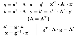








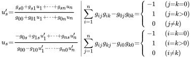













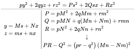


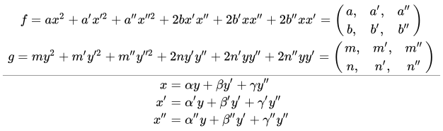

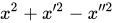



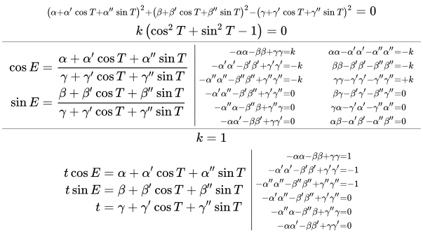
![{\displaystyle [\cos T,\sin T,\cos E,\sin E]=\left[u_{1},\ u_{2},\ u_{1}^{\prime },\ u_{2}^{\prime }\right]}](https://wikimedia.org/api/rest_v1/media/math/render/svg/eababb1457efc2ccf349777160c8316d35c8a5b8)




![{\displaystyle \left[\cos T,\sin T,\cos E,\sin E\right]=\left[{\tfrac {x}{z}},\ {\tfrac {y}{z}},\ {\tfrac {u'}{u}},\ {\tfrac {u''}{u}}\right]}](https://wikimedia.org/api/rest_v1/media/math/render/svg/b6275156c23d62ea353e95df35f9607b66757ede)

![{\displaystyle {\scriptstyle {\begin{aligned}\left[\cos P,\ \sin P\cos \varphi ,\ \sin P\sin \varphi \right]&=\left[u_{1},\ u_{2},\ u_{3}\right]\\{}[\cos \psi ,\ \sin \psi \cos \vartheta ,\ \sin \psi \sin \vartheta ]&=\left[u_{1}^{\prime },\ u_{2}^{\prime },\ u_{3}^{\prime }\right]\end{aligned}}}}](https://wikimedia.org/api/rest_v1/media/math/render/svg/440ef9f3590b69cfd3cd55f9d28f924c0e67edc2)

![{\displaystyle {\scriptstyle {\begin{matrix}xx+yy+zz=ss+s's'+s''s''=0\\\mathbf {(1)} {\begin{aligned}x&=\alpha s+\alpha 's'+\alpha ''s''\\y&=\beta s+\beta 's'+\beta ''s''\\z&=\gamma s+\gamma 's'+\gamma ''s''\\\\s&=\alpha x+\beta y+\gamma z\\s'&=\alpha 'x+\beta 'y+\gamma 'z\\s''&=\alpha ''x+\beta ''y+\gamma ''z\end{aligned}}\left|{\begin{aligned}\alpha \alpha +\beta \beta +\gamma \gamma &=1&\alpha \alpha +\alpha '\alpha '+\alpha ''\alpha ''&=1\\\alpha '\alpha '+\beta '\beta '+\gamma '\gamma '&=1&\beta \beta +\beta '\beta '+\beta ''\beta ''&=1\\\alpha ''\alpha ''+\beta ''\beta ''+\gamma ''\gamma ''&=1&\gamma \gamma +\gamma '\gamma '+\gamma ''\gamma ''&=1\\\alpha '\alpha ''+\beta '\beta ''+\gamma '\gamma ''&=0&\beta \gamma +\beta '\gamma '+\beta ''\gamma ''&=0\\\alpha ''\alpha +\beta ''\beta +\gamma ''\gamma &=0&\gamma \alpha +\gamma '\alpha '+\gamma ''\alpha ''&=0\\\alpha \alpha '+\beta \beta '+\gamma \gamma '&=0&\alpha \beta +\alpha '\beta '+\alpha ''\beta ''&=0\end{aligned}}\right.\\\hline \left[{\frac {y}{x}},\ {\frac {z}{x}},\ {\frac {s'}{s}},\ {\frac {s''}{s}}\right]=\left[-i\cos \varphi ,\ -i\sin \varphi ,\ i\cos \eta ,\ i\sin \eta \right]\\\left[\alpha ',\ \alpha '',\ \beta ,\ \gamma \right]=\left[i\alpha ',\ i\alpha '',\ -i\beta ,\ -i\gamma \right]\\\hline {\begin{matrix}\mathbf {(2)} {\begin{matrix}\left(\alpha -\alpha '\cos \eta -\alpha ''\sin \eta \right)^{2}=\left(\beta -\beta '\cos \eta -\beta ''\sin \eta \right)^{2}+\left(\gamma -\gamma '\cos \eta -\gamma ''\sin \eta \right)^{2}\\\left(\alpha -\beta \cos \phi -\gamma \sin \phi \right)^{2}=\left(\alpha '-\beta '\cos \phi -\gamma '\sin \phi \right)^{2}+\left(\alpha ''-\beta ''\cos \phi -\gamma ''\sin \phi \right)^{2}\\\hline {\begin{aligned}\cos \phi &={\frac {\beta -\beta '\cos \eta -\beta ''\sin \eta }{\alpha -\alpha '\cos \eta -\alpha ''\sin \eta }},&\cos \eta &={\frac {\alpha '-\beta '\cos \phi -\gamma '\sin \phi }{\alpha -\beta \cos \phi -\gamma \sin \phi }}\\\sin \phi &={\frac {\gamma -\gamma '\cos \eta -\gamma ''\sin \eta }{\alpha -\alpha '\cos \eta -\alpha ''\sin \eta }},&\sin \eta &={\frac {\alpha ''-\beta ''\cos \phi -\gamma ''\sin \phi }{\alpha -\beta \cos \phi -\gamma \sin \phi }}\end{aligned}}\end{matrix}}\\\hline \\\mathbf {(3)} {\begin{matrix}1-zz-yy={\frac {1-s's'-s''s''}{\left(\alpha -\alpha 's'-\alpha ''s''\right)^{2}}}\\\hline {\begin{aligned}y&={\frac {\beta -\beta 's'-\beta ''s''}{\alpha -\alpha 's'-\alpha ''s''}},&s'&={\frac {\alpha '-\beta 'y-\gamma 'z}{\alpha -\beta y-\gamma z}},\\z&={\frac {\gamma -\gamma 's'-\gamma ''s''}{\alpha -\alpha 's'-\alpha ''s'''}},&s''&={\frac {\alpha ''-\beta ''y-\gamma ''z}{\alpha -\beta y-\gamma z}},\end{aligned}}\end{matrix}}\end{matrix}}\left|{\begin{aligned}\alpha \alpha -\beta \beta -\gamma \gamma &=1\\\alpha '\alpha '-\beta '\beta '-\gamma '\gamma '&=-1\\\alpha ''\alpha ''-\beta ''\beta ''-\gamma ''\gamma ''&=-1\\\alpha '\alpha ''-\beta '\beta ''-\gamma '\gamma ''&=0\\\alpha ''\alpha -\beta ''\beta -\gamma ''\gamma &=0\\\alpha \alpha '-\beta \beta '-\gamma \gamma '&=0\\\\\alpha \alpha -\alpha '\alpha '-\alpha ''\alpha ''&=1\\\beta \beta -\beta '\beta '-\beta ''\beta ''&=-1\\\gamma \gamma -\gamma '\gamma '-\gamma ''\gamma ''&=-1\\\beta \gamma -\beta '\gamma '-\beta ''\gamma ''&=0\\\gamma \alpha -\gamma '\alpha '-\gamma ''\alpha ''&=0\\\alpha \beta -\alpha '\beta '-\alpha ''\beta ''&=0\end{aligned}}\right.\end{matrix}}}}](https://wikimedia.org/api/rest_v1/media/math/render/svg/78cf107c14b543adef885acdd0559bb611eb7fb3)
![{\displaystyle [\cos \phi ,\ \sin \phi ,\ \cos \eta ,\ \sin \eta ]=\left[u_{1},\ u_{2},\ u_{1}^{\prime },\ u_{2}^{\prime }\right]}](https://wikimedia.org/api/rest_v1/media/math/render/svg/16e7353553eb2ba432da8c57c41f666d3049f67e)
![{\displaystyle {\scriptstyle {\begin{matrix}x_{1}x_{1}+x_{2}x_{2}+\dots +x_{n}x_{n}=y_{1}y_{1}+y_{2}y_{2}+\dots +y_{n}y_{n}\\\hline \mathbf {(1)\ } {\begin{aligned}y_{\varkappa }&=\alpha _{1}^{(\varkappa )}x_{1}+\alpha _{2}^{(\varkappa )}x_{2}+\dots +\alpha _{n}^{(\varkappa )}x_{n}\\x_{\varkappa }&=\alpha _{\varkappa }^{\prime }y_{1}+\alpha _{\varkappa }^{\prime \prime }y_{2}+\dots +\alpha _{\varkappa }^{(n)}y_{n}\\\\{\frac {y_{\varkappa }}{y_{n}}}&={\frac {\alpha _{1}^{(\varkappa )}x_{1}+\alpha _{2}^{(\varkappa )}x_{2}+\dots +\alpha _{n}^{(\varkappa )}x_{n}}{\alpha _{1}^{(n)}x_{1}+\alpha _{2}^{(n)}x_{2}+\dots +\alpha _{n}^{(n)}x_{n}}}\\{\frac {x_{\varkappa }}{x_{n}}}&={\frac {\alpha _{\varkappa }^{\prime }y_{1}+\alpha _{\varkappa }^{\prime \prime }y_{2}+\dots +\alpha _{\varkappa }^{(n)}y_{n}}{\alpha _{1}^{(n)}x_{1}+\alpha _{2}^{(n)}x_{2}+\dots +\alpha _{n}^{(n)}x_{n}}}\end{aligned}}\left|{\begin{aligned}\alpha _{\varkappa }^{\prime }\alpha _{\lambda }^{\prime }+\alpha _{\varkappa }^{\prime \prime }\alpha _{\lambda }^{\prime \prime }+\dots +\alpha _{\varkappa }^{(n)}\alpha _{\lambda }^{(n)}&=0\\\alpha _{\varkappa }^{\prime }\alpha _{\varkappa }^{\prime }+\alpha _{\varkappa }^{\prime \prime }\alpha _{\varkappa }^{\prime \prime }+\dots +\alpha _{\varkappa }^{(n)}\alpha _{\varkappa }^{(n)}&=1\\\\\alpha _{1}^{(\varkappa )}\alpha _{1}^{(\lambda )}+\alpha _{2}^{(\varkappa )}\alpha _{2}^{(\lambda )}+\dots +\alpha _{n}^{(\varkappa )}\alpha _{n}^{(\lambda )}&=0\\\alpha _{1}^{(\varkappa )}\alpha _{1}^{(\varkappa )}+\alpha _{2}^{(\varkappa )}\alpha _{2}^{(\varkappa )}+\dots +\alpha _{n}^{(\varkappa )}\alpha _{n}^{(\varkappa )}&=1\end{aligned}}\right.\\\hline {\frac {x_{\varkappa }}{x_{n}}}=-i\xi _{\varkappa },\ {\frac {y_{\varkappa }}{y_{n}}}=i\nu _{\varkappa }\\1-\xi _{1}\xi _{1}-\xi _{2}\xi _{2}-\dots -\xi _{n-1}\xi _{n-1}={\frac {y_{n}y_{n}}{x_{n}x_{n}}}\left(1-\nu _{1}\nu _{1}-\nu _{2}\nu _{2}-\dots -\nu _{n-1}\nu _{n-1}\right)\\\alpha _{n}^{(\varkappa )}=i\alpha ^{(\varkappa )},\ \alpha _{\varkappa }^{(n)}=-i\alpha _{\varkappa },\ \alpha _{n}^{(n)}=\alpha \\1-\xi _{1}\xi _{1}-\xi _{2}\xi _{2}-\dots -\xi _{n-1}\xi _{n-1}={\frac {1-\nu _{1}\nu _{1}-\nu _{2}\nu _{2}-\dots -\nu _{n-1}\nu _{n-1}}{\left[\alpha -\alpha ^{\prime }\nu _{1}-\alpha ^{\prime \prime }\nu _{2}\dots -\alpha ^{(n-1)}\nu _{n-1}\right]^{2}}}\\\hline \mathbf {(2)\ } {\begin{aligned}\nu _{\varkappa }&={\frac {\alpha ^{(\varkappa )}-\alpha _{1}^{(\varkappa )}\xi _{1}-\alpha _{2}^{(\varkappa )}\xi _{2}\dots -\alpha _{n-1}^{(\varkappa )}\xi _{n-1}}{\alpha -\alpha _{1}\xi _{1}-\alpha _{2}\xi _{2}\dots -\alpha _{n-1}\xi _{n-1}}}\\\\\xi _{\varkappa }&={\frac {\alpha _{\varkappa }-\alpha _{\varkappa }^{\prime }\nu _{1}-\alpha _{2}^{\prime \prime }\nu _{2}\dots -\alpha _{\varkappa }^{(n-1)}\nu _{n-1}}{\alpha -\alpha ^{\prime }\nu _{1}-\alpha ^{\prime \prime }\nu _{2}\dots -\alpha ^{(n-1)}\nu _{n-1}}}\end{aligned}}\\\hline \xi _{1}\xi _{1}-\xi _{2}\xi _{2}-\dots -\xi _{n-1}\xi _{n-1}=1\ \Rightarrow \ \nu _{1}\nu _{1}-\nu _{2}\nu _{2}-\dots -\nu _{n-1}\nu _{n-1}=1\end{matrix}}}}](https://wikimedia.org/api/rest_v1/media/math/render/svg/0ace40fa624402c009247e2c1a88467d67e871af)
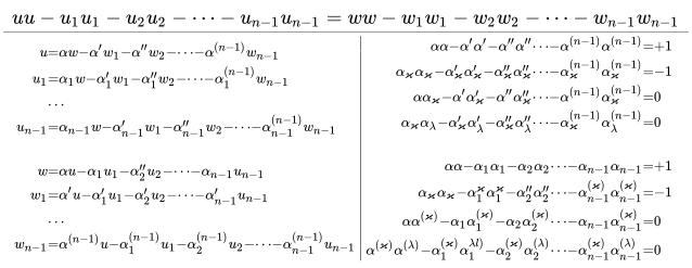
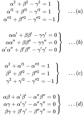
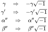
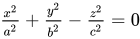
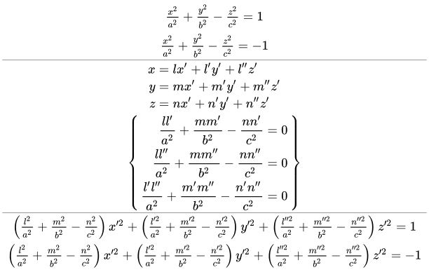

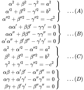
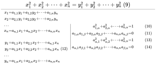

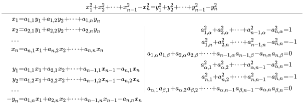
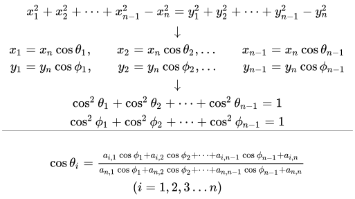
![{\displaystyle [\cos \theta _{i},\ \cos \phi _{i}]=\left[u_{s},\ u_{s}^{\prime }\right]}](https://wikimedia.org/api/rest_v1/media/math/render/svg/68b56c344e5dd459b84f7795caa7682dafedc9f1)
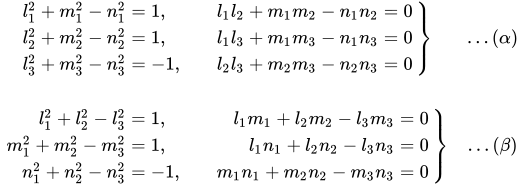

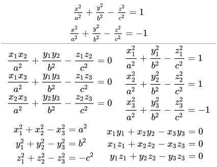
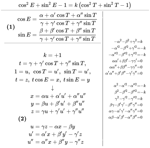
![{\displaystyle [k,\cos T,\sin T,\cos E,\sin E]=\left[1,u_{1},u_{2},u_{1}^{\prime },u_{2}^{\prime }\right]}](https://wikimedia.org/api/rest_v1/media/math/render/svg/d3a539dec17c64c12fc762d268cfee49fd030285)
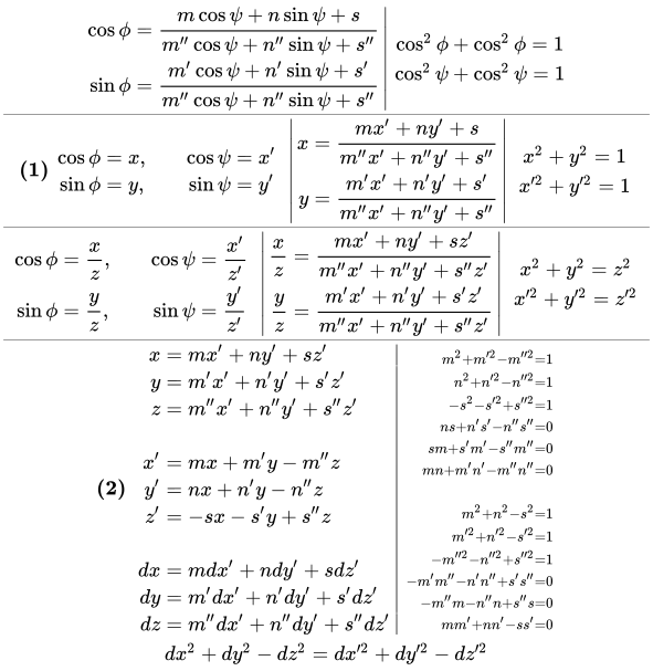





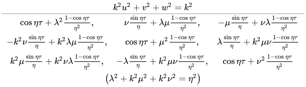
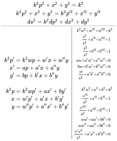
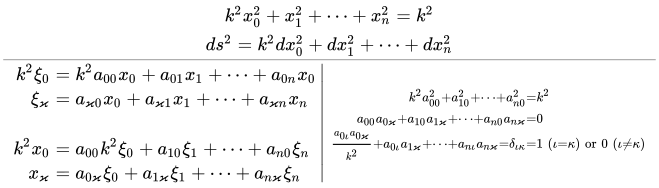


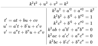
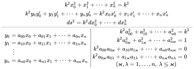
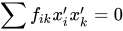
![{\displaystyle {\begin{matrix}x_{1}^{2}+\dots +x_{m+1}^{2}=1\\\hline X_{\iota \varkappa }f=x_{i}{\frac {\partial f}{\partial x_{\varkappa }}}-x_{\varkappa }{\frac {\partial f}{\partial x_{\iota }}}\\{\text{where}}\\\left(X_{\iota \varkappa },X_{\iota \lambda }\right)=X_{\varkappa \lambda };\ \left(X_{\iota \varkappa },X_{\lambda \mu }\right)=0;\\\left[\iota \neq \varkappa \neq \lambda \neq \mu \right]\end{matrix}}}](https://wikimedia.org/api/rest_v1/media/math/render/svg/b6f370afcafbb76456ca494048813686fc85db57)
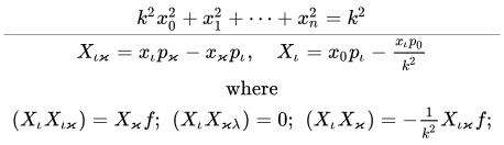

![{\displaystyle {\begin{matrix}{\begin{matrix}k^{2}x_{0}^{2}+x_{1}^{2}+\dots +x_{n}^{2}&(a)\\k^{2}x_{0}^{2}+x_{1}^{2}+\dots +x_{n}^{2}=k^{2}&(b)\end{matrix}}\\\hline V_{\varkappa }=k^{2}x_{0}p_{\varkappa }-x_{\varkappa }p_{0},\quad U_{\iota \varkappa }=p_{\iota }x_{\varkappa }-p_{\varkappa }x_{\iota }\\{\text{where}}\\\left(V_{\iota },V_{\varkappa }\right)=k^{2}U_{\iota \varkappa },\ \left(V_{\iota },U_{\iota \varkappa }\right)=-V_{\varkappa },\ \left(V_{\iota },U_{\varkappa \lambda }\right)=0,\\\left(U_{\iota \varkappa },U_{\iota \lambda }\right)=U_{\varkappa \lambda },\ \left(U_{\iota \varkappa },U_{\lambda \mu }\right)=0\\\left[\iota ,\varkappa ,\lambda ,\mu =1,2,\dots n\right]\\\hline {\begin{matrix}y_{1}={\frac {x_{1}}{x_{0}}},\ y_{2}={\frac {x_{2}}{x_{0}}},\dots y_{n}={\frac {x_{n}}{x_{0}}}\\\downarrow \\k^{2}+y_{1}^{2}+y_{2}^{2}+\dots +y_{n}^{2}=0\\\hline q_{\varkappa }+{\frac {y_{\varkappa }}{k^{2}}}\sum _{\varrho }y_{y}q_{\varrho },\quad q_{\iota }y_{\varkappa }-q_{\varkappa }y_{\iota }\end{matrix}}\end{matrix}}}](https://wikimedia.org/api/rest_v1/media/math/render/svg/6d115e3c538573d4a0098ae23a6ba76908104bce)
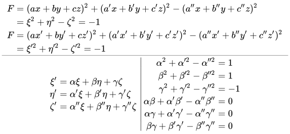
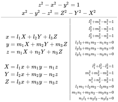




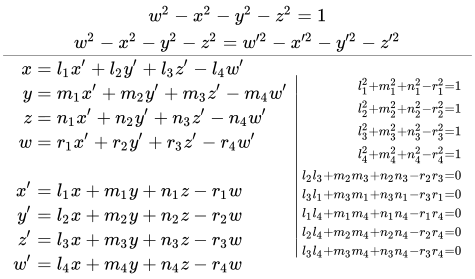
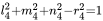


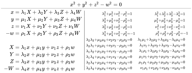


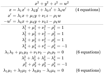
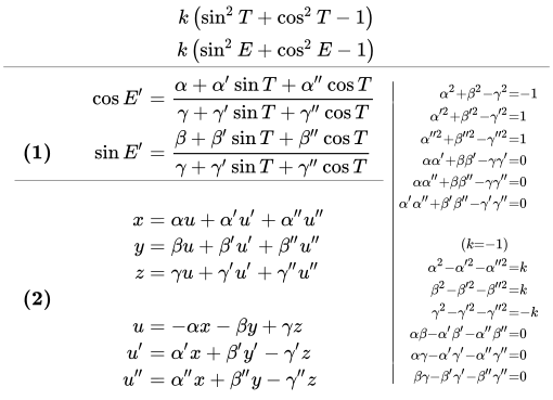
![{\displaystyle [\cos T,\sin T,\cos E',\sin E']=\left[u_{1},u_{2},u_{1}^{\prime },u_{2}^{\prime }\right]}](https://wikimedia.org/api/rest_v1/media/math/render/svg/a71c6cad65b9e62f5fb4f84f9053ac2869e4069f)
![{\displaystyle {\begin{matrix}{\begin{matrix}xx_{0}+yy_{0}-zz_{0}\\\\\mathbf {(1)} \ {\begin{aligned}x&=M_{1}X+P_{1}Y+R_{1}Z\\y&=M_{2}X+P_{2}Y+R_{2}Z\\z&=M_{3}X+P_{3}Y+R_{3}Z\end{aligned}}\\\\\left[{\begin{aligned}[][x,y,z]={\text{complex}}\\\left[x_{0},y_{0},z_{0}\right]={\text{conjugate}}\end{aligned}}\right]\\\\\hline \\x^{\prime 2}+x^{\prime \prime 2}+y^{\prime 2}+y^{\prime \prime 2}=1\\x=x'+ix'',\quad y=y'+iy''\\\\\mathbf {(2)} \ {\begin{aligned}X&={\frac {M_{1}x+P_{1}y+R_{1}}{M_{3}x+P_{3}y+R_{3}}}\\Y&={\frac {M_{2}x+P_{2}y+R_{2}}{M_{3}x+P_{3}y+R_{3}}}\end{aligned}}\end{matrix}}\left|{\scriptstyle {\begin{aligned}M_{1}\mu _{1}+M_{2}\mu _{2}-M_{3}\mu _{3}&=1\\P_{1}\pi _{1}+P_{2}\pi _{2}-P_{3}\pi _{3}&=1\\R_{1}\rho _{1}+R_{2}\rho _{2}-R_{3}\rho _{3}&=-1\\P_{1}\mu _{1}+P_{2}\mu _{2}-P_{3}\mu _{3}&=0\\M_{1}\rho _{1}+M_{2}\rho _{2}-M_{3}\rho _{3}&=0\\P_{1}\rho _{1}+P_{2}\rho _{2}-P_{3}\rho _{3}&=0\\\\M_{1}\mu _{1}+P_{1}\pi _{1}-R_{1}\rho _{1}&=1\\M_{2}\mu _{2}+P_{2}\pi _{2}-R_{2}\rho _{2}&=1\\M_{3}\mu _{3}+P_{3}\pi _{3}-R_{3}\rho _{3}&=-1\\\mu _{2}M_{1}+\pi _{2}P_{1}-R_{1}\rho _{2}&=0\\\mu _{2}M_{3}+\pi _{2}P_{3}-R_{3}\rho _{2}&=0\\\mu _{3}M_{1}+\pi _{3}P_{1}-R_{1}\rho _{3}&=0\\\\\left[{\begin{aligned}[][M,P,R\dots ]={\text{complex}}\\\left[\mu ,\pi ,\rho \dots \right]={\text{conjugate}}\end{aligned}}\right]\end{aligned}}}\right.\end{matrix}}}](https://wikimedia.org/api/rest_v1/media/math/render/svg/059d4ad5c99a9cd0684e2a092888988359bbfdf2)
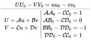
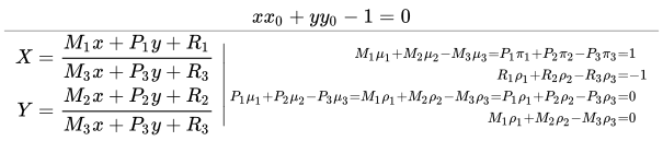
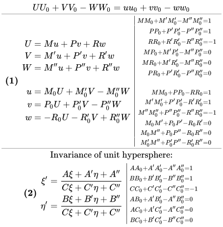

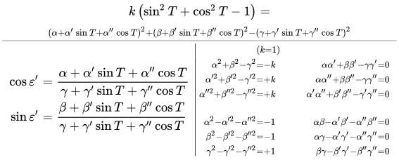
![{\displaystyle [\cos T,\sin T,\cos \varepsilon ',\sin \varepsilon ']=\left[u_{1},u_{2},u_{1}^{\prime },u_{2}^{\prime }\right]}](https://wikimedia.org/api/rest_v1/media/math/render/svg/523f090452a3187b5fb29c15a07bd1ed9a86a770)
![{\displaystyle {\begin{matrix}x_{1}^{2}+x_{2}^{2}+\dots +x_{n}^{2}=1\\\hline x_{i}p_{\varkappa }-x_{\varkappa }p_{i},\quad p_{i}-x_{i}\sum _{1}^{n}{\scriptstyle j}\ x_{j}p_{j}\quad (i,\varkappa =1,\dots ,n)\\{\text{where}}\\\left(Q_{i},Q_{\varkappa }\right)=R_{i,\varkappa };\ \left(Q_{i},Q_{j,\varkappa }\right)=\varepsilon _{i,j}Q_{\varkappa }-\varepsilon _{i,\varkappa }Q_{j};\\\left(R_{i,\varkappa },R_{\mu ,\nu }\right)=\varepsilon _{\varkappa ,\mu }R_{i,\nu }-\varepsilon _{\varkappa ,\nu }R_{i,\mu }-\varepsilon _{,\mu }R_{\varkappa ,\nu }+\varepsilon _{i,\nu }R_{\varkappa ,\mu }\\\left[\varepsilon _{i,\varkappa }\equiv 0\ {\text{for}}\ i\neq \varkappa ;\ \varepsilon _{i,i}=1\right]\end{matrix}}}](https://wikimedia.org/api/rest_v1/media/math/render/svg/77a7e3d5f0435c2831419b41518e7a8e76e37046)