Waves in composites and metamaterials/Bloch waves and the quasistatic limit

From Wikiversity

[edit] Bloch Theorem

In the previous lecture we showed that Maxwell's equations at fixed frequency can be formulated in terms of the fields $\mathbf{D}$ and $\mathbf{B}$ as ^[1]

$\text{(1)} \qquad \boldsymbol{\nabla} \cdot \mathbf{D} = 0 ~;~~ \boldsymbol{\nabla} \cdot \mathbf{B} = 0 ~;~~ i~\boldsymbol{\nabla} \times \left(\cfrac{\mathbf{D}}{\epsilon}\right) = \omega~\mathbf{B} ~;~~ -i~\boldsymbol{\nabla} \times \left(\cfrac{\mathbf{B}}{\mu}\right) = \omega~\mathbf{D} ~.$

Equations (1) suggest that we should look for solutions $\mathbf{D}$ and $\mathbf{B}$ in the space of divergence-free fields such that

$\text{(2)} \qquad \mathcal{L}\begin{bmatrix} \mathbf{D} \\ \mathbf{B} \end{bmatrix} = \omega~\begin{bmatrix} \mathbf{D} \\ \mathbf{B} \end{bmatrix} \qquad \text{or} \qquad { (\mathcal{L} - \omega~\boldsymbol{1})\begin{bmatrix}\mathbf{D} \\ \mathbf{B} \end{bmatrix} = \boldsymbol{0} }$

where the operator $\mathcal{L}$ is given by

$\text{(3)} \qquad { \mathcal{L} := \begin{bmatrix} 0 & -i~\boldsymbol{\nabla} \times \mu^{-1} \\ i~\boldsymbol{\nabla} \times \epsilon^{-1} & 0 \end{bmatrix} ~. }$

If the medium is such that the permittivity $\epsilon(\mathbf{x})$ and the permeability $\mu(\mathbf{x})$ are periodic, i.e.,

$\epsilon(\mathbf{x}) = \epsilon(\mathbf{x} + \mathbf{R}) ~;~~ \mu(\mathbf{x}) = \mu(\mathbf{x} + \mathbf{R})$

where $\mathbf{R}$ is a lattice vector (see Figure 1) then the operator $\mathcal{L}$ has the same periodicity as the medium.

Figure 1. Lattice vector in a periodic medium.

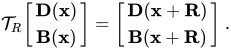
Also recall the translation operator $\mathcal{T}_R$ defined as

${ \mathcal{T}_R\begin{bmatrix} \mathbf{D}(\mathbf{x}) \\ \mathbf{B}(\mathbf{x}) \end{bmatrix} = \begin{bmatrix} \mathbf{D}(\mathbf{x}+\mathbf{R}) \\ \mathbf{B}(\mathbf{x}+\mathbf{R}) \end{bmatrix} ~. }$

Periodicity of the medium implies that $\mathcal{T}_R$ commutes with $\mathcal{L}$ , i.e.,

${ \mathcal{T}_R~\mathcal{L} = \mathcal{L}~\mathcal{T}_R ~. }$

^[2] The translation operator is unitary, i.e.,

${ \mathcal{T}_R~\mathcal{T}_R^T = \mathcal{T}_R~\mathcal{T}_{-R} = \boldsymbol{1} ~. }$

This means that the adjoint operator $\mathcal{T}_R^T$ is equal to the inverse operator $\mathcal{T}_{-R}$ .

The translation operator also commutes, i.e.,

${ \mathcal{T}_R~\mathcal{T}_{R'} = \mathcal{T}_{R'}~\mathcal{T}_R = \mathcal{T}_{R+R'} ~. }$

^[3] Also, since $\mathcal{L}$ and $\mathcal{T}_R$ commute, the operators $\mathcal{L}-\omega\boldsymbol{1}$ and $\mathcal{T}_R$ must also commute. This implies that

$\mathcal{T}_R~(\mathcal{L} - \omega~\boldsymbol{1}) ~\begin{bmatrix}\mathbf{D}(\mathbf{x}) \\ \mathbf{B}(\mathbf{x})\end{bmatrix} = \boldsymbol{0} = (\mathcal{L} - \omega~\boldsymbol{1})~\mathcal{T}_R ~\begin{bmatrix}\mathbf{D}(\mathbf{x}) \\ \mathbf{B}(\mathbf{x})\end{bmatrix} = (\mathcal{L} - \omega~\boldsymbol{1})~ ~\begin{bmatrix}\mathbf{D}(\mathbf{x}+\mathbf{R}) \\ \mathbf{B}(\mathbf{x}+\mathbf{R})\end{bmatrix} ~.$

Hence the eigenstates of $\mathcal{L} - \omega~\boldsymbol{1}$ and the eigenstates of $\mathcal{T}_R$ lie in the same space. Therefore, any solution can be expressed in fields which are simultaneously eigenstates of all the $\mathcal{T}_R$ , i.e., these eigenstates have the property

$\text{(4)} \qquad { [\mathcal{T}_R - c(\mathbf{R})~\boldsymbol{1}]\begin{bmatrix} \mathbf{D}(\mathbf{x}) \\ \mathbf{B}(\mathbf{x}) \end{bmatrix} = \boldsymbol{0} ~. }$

Since $\mathcal{T}_R~\mathcal{T}_{R'} = \mathcal{T}_{R+R'}$ , we have

$c(\mathbf{R})~c(\mathbf{R}') = c(\mathbf{R} + \mathbf{R}') ~.$

So it suffices to know $c(\mathbf{R})$ when $\mathbf{R} = \mathbf{a}_1, \mathbf{a}_2 , \mathbf{a}_3$ where the $\mathbf{a}_i$ 's are the primitive vectors of the lattice, i.e.,

$\epsilon(\mathbf{x} + \mathbf{a}_j) = \epsilon(\mathbf{x}) ~;~~ \mu(\mathbf{x} + \mathbf{a}_j) = \mu(\mathbf{x}) ~.$

Let us assume that

$c(\mathbf{a}_j) = e^{2\pi~i~\alpha_j} \qquad j = 1, 2, 3$

for a suitable choice of $α j$ .

Then for any lattice vector

$\mathbf{R} = n_1~\mathbf{a}_1 + n_2~\mathbf{a}_2 + n_3~\mathbf{a}_3$

we have

$\begin{align} c(\mathbf{R}) & = c(n_1~\mathbf{a}_1 + n_2~\mathbf{a}_2 + n_3~\mathbf{a}_3) = c(n_1~\mathbf{a}_1)~c(n_2~\mathbf{a}_2)~c(n_3~\mathbf{a}_3) \\ & = c\left(\sum_{i=1}^{n_1}\mathbf{a}_1\right)~ c\left(\sum_{i=1}^{n_2}\mathbf{a}_2\right)~c\left(\sum_{i=1}^{n_3}\mathbf{a}_3\right) = [c(\mathbf{a}_1)]^{n_1}~[c(\mathbf{a}_2)]^{n_2}~[c(\mathbf{a}_3)]^{n_3} \\ & = e^{2\pi i \alpha_1~n_1}~e^{2\pi i \alpha_2~n_2}~e^{2\pi i \alpha_3~n_3} = e^{2\pi i (\alpha_1~n_1 + \alpha_2~n_2 + \alpha_3~n_3)} \end{align}$

or,

$c(\mathbf{R}) = e^{2\pi i (\alpha_1~n_1 + \alpha_2~n_2 + \alpha_3~n_3)} ~.$

Define a vector

$\mathbf{k} := \alpha_1~\mathbf{b}_1 + \alpha_2~\mathbf{b}_2 + \alpha_3~\mathbf{b}_3$

where the vectors $\mathbf{b}_i$ are the reciprocal lattice vectors satisfying

$\mathbf{b}_i\cdot\mathbf{a}_j = 2\pi~\delta_{ij} ~.$

Then,

$\mathbf{k}\cdot\mathbf{R} = (\alpha_1~\mathbf{b}_1 + \alpha_2~\mathbf{b}_2 + \alpha_3~\mathbf{b}_3) \cdot (n_1~\mathbf{a}_1 + n_2~\mathbf{a}_2 + n_3~\mathbf{a}_3) = \alpha_1~n_1~2~\pi + \alpha_2~n_2~2~\pi + \alpha_3~n_3~2~\pi$

or,

$\mathbf{k}\cdot\mathbf{R} = 2\pi (\alpha_1~n_1 + \alpha_2~n_2 + \alpha_3~n_3) ~.$

Therefore, we have

$c(\mathbf{R}) = e^{i \mathbf{k}\cdot\mathbf{R}} ~.$

Plugging this expression into (4), we get

$[\mathcal{T}_R - e^{i \mathbf{k}\cdot\mathbf{R}}~\boldsymbol{1}] \begin{bmatrix} \mathbf{D}(\mathbf{x}) \\ \mathbf{B}(\mathbf{x}) \end{bmatrix} = \boldsymbol{0}$

or,

$\text{(5)} \qquad { \begin{bmatrix} \mathbf{D}(\mathbf{x}+\mathbf{R}) \\ \mathbf{B}(\mathbf{x}+\mathbf{R}) \end{bmatrix} = e^{i \mathbf{k}\cdot\mathbf{R}}~ \begin{bmatrix} \mathbf{D}(\mathbf{x}) \\ \mathbf{B}(\mathbf{x}) \end{bmatrix} ~. }$

Equation (5) is called the Bloch condition.

In summary, the solutions to the electromagnetic equations in a periodic medium can be expressed in Bloch waves where each Bloch wave is a time harmonic solution to the electromagnetic equations which in addition satisfies the Bloch condition for all lattice vectors $\mathbf{R}$ and for some appropriate choice of $\mathbf{k}$ .

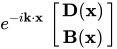
Note that for any vector $\mathbf{x}$ , the Bloch condition implies that

$e^{-i \mathbf{k}\cdot(\mathbf{x}+\mathbf{R})} \begin{bmatrix} \mathbf{D}(\mathbf{x}+\mathbf{R}) \\ \mathbf{B}(\mathbf{x}+\mathbf{R}) \end{bmatrix} = e^{i \mathbf{k}\cdot\mathbf{R} - i \mathbf{k} \cdot\mathbf{R} - i \mathbf{k} \cdot \mathbf{x}}~ \begin{bmatrix} \mathbf{D}(\mathbf{x}) \\ \mathbf{B}(\mathbf{x}) \end{bmatrix} = e^{- i \mathbf{k} \cdot \mathbf{x}}~ \begin{bmatrix} \mathbf{D}(\mathbf{x}) \\ \mathbf{B}(\mathbf{x}) \end{bmatrix} ~.$

Therefore the quantity

$e^{- i \mathbf{k} \cdot \mathbf{x}}~ \begin{bmatrix} \mathbf{D}(\mathbf{x}) \\ \mathbf{B}(\mathbf{x}) \end{bmatrix}$

is periodic.

[edit] Quasistatic Limit

Let us now consider the solution of Maxwell's equation in periodic media in the quasistatic limit. ^[4] Consider the periodic medium shown in Figure 2. The lattice spacing is $η$ .

Figure 2. Periodic medium with

x

and

y

spaces.

Define

$\epsilon_\eta(\mathbf{x}) := \epsilon\left(\cfrac{\mathbf{x}}{\eta}\right) = \epsilon(\mathbf{y})~;~~ \mu_\eta(\mathbf{x}) := \mu\left(\cfrac{\mathbf{x}}{\eta}\right) = \mu(\mathbf{y}) ~.$

These are periodic functions, i.e.,

$\epsilon(\mathbf{y} + \mathbf{a}_i) = \epsilon(\mathbf{y}) ~;~~ \mu(\mathbf{y} + \mathbf{a}_i) = \mu(\mathbf{y})$

where $\mathbf{a}_i$ are the primitive lattice vectors. We may also write these periodicity conditions as

$\epsilon_\eta(\mathbf{x} + \eta\mathbf{a}_i) = \epsilon_\eta(\mathbf{x}) ~;~~ \mu_\eta(\mathbf{x} + \eta\mathbf{a}_i) = \mu_\eta(\mathbf{x}) ~.$

Similarly, define

$\mathbf{D}_\eta(\mathbf{x}) := \mathbf{D}(\mathbf{y}) ~;~~ \mathbf{B}_\eta(\mathbf{x}) := \mathbf{B}(\mathbf{y}) ~;~~ \mathbf{E}_\eta(\mathbf{x}) := \mathbf{E}(\mathbf{y}) ~;~~ \mathbf{H}_\eta(\mathbf{x}) := \mathbf{H}(\mathbf{y}) ~.$

Then Maxwell's equations can be written as

$\text{(6)} \qquad \boldsymbol{\nabla} \cdot \mathbf{D}_\eta = 0 ~;~~ \boldsymbol{\nabla} \cdot \mathbf{B}_\eta = 0 ~;~~ \boldsymbol{\nabla} \times \mathbf{E}_\eta - i\omega~\mathbf{B}_\eta = \boldsymbol{0} ~;~~ \boldsymbol{\nabla} \times \mathbf{H}_\eta + i\omega~\mathbf{D}_\eta = \boldsymbol{0} ~.$

Let us look for Bloch wave solutions of the form

$\mathbf{E}_\eta(\mathbf{x}) = e^{i\mathbf{k}\cdot\mathbf{x}}~\mathbf{e}_\eta(\mathbf{x}) ~;~~ \mathbf{D}_\eta(\mathbf{x}) = e^{i\mathbf{k}\cdot\mathbf{x}}~\mathbf{d}_\eta(\mathbf{x}) ~;~~ \mathbf{H}_\eta(\mathbf{x}) = e^{i\mathbf{k}\cdot\mathbf{x}}~\mathbf{h}_\eta(\mathbf{x}) ~;~~ \mathbf{B}_\eta(\mathbf{x}) = e^{i\mathbf{k}\cdot\mathbf{x}}~\mathbf{b}_\eta(\mathbf{x})$

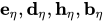
where $\mathbf{e}_\eta, \mathbf{d}_\eta, \mathbf{h}_\eta, \mathbf{b}_\eta$ have the same periodicity as $ε$ and $μ$ , i.e.,

$\mathbf{e}_\eta(\mathbf{x} + \eta~\mathbf{a}_i) = \mathbf{e}(\mathbf{x}) ~;~~ \mathbf{d}_\eta(\mathbf{x} + \eta~\mathbf{a}_i) = \mathbf{d}(\mathbf{x}) ~;~~ \mathbf{h}_\eta(\mathbf{x} + \eta~\mathbf{a}_i) = \mathbf{h}(\mathbf{x}) ~;~~ \mathbf{b}_\eta(\mathbf{x} + \eta~\mathbf{a}_i) = \mathbf{b}(\mathbf{x}) ~.$

From the constitutive relations, we get

$\mathbf{d}_\eta(\mathbf{x}) = \epsilon_\eta(\mathbf{x})~\mathbf{e}_\eta(\mathbf{x}) ~;~~ \mathbf{b}_\eta(\mathbf{x}) = \mu_\eta(\mathbf{x})~\mathbf{h}_\eta(\mathbf{x}) ~.$

Recall that, for periodic media, Maxwell's equations may be expressed as

$(\mathcal{L} - \omega~\boldsymbol{1})\begin{bmatrix}\mathbf{D} \\ \mathbf{B} \end{bmatrix} = \boldsymbol{0} ~.$

Here $ω$ is an eigenvalue of $\mathcal{L}$ . However, $\mathcal{L}$ depends on $ω$ via $ε(ω)$ and $μ(ω)$ . {\bf Bloch wave solutions do not exists unless $ω$ takes one of a discrete set of values.}

Let these discrete values be

$\omega = \omega_\eta^j(\mathbf{k})$

where the superscript $j$ labels the solution branches.

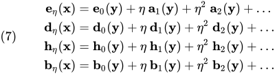
Let us see what the Bloch wave solutions reduce to as $\eta\rightarrow 0$ . Following standard multiple scale analysis, let us assume that the periodic complex fields have the expansions

$\text{(7)} \qquad \begin{align} \mathbf{e}_\eta(\mathbf{x}) & = \mathbf{e}_0(\mathbf{y}) + \eta~\mathbf{a}_1(\mathbf{y}) + \eta^2~\mathbf{a}_2(\mathbf{y}) + \dots \\ \mathbf{d}_\eta(\mathbf{x}) & = \mathbf{d}_0(\mathbf{y}) + \eta~\mathbf{d}_1(\mathbf{y}) + \eta^2~\mathbf{d}_2(\mathbf{y}) + \dots \\ \mathbf{h}_\eta(\mathbf{x}) & = \mathbf{h}_0(\mathbf{y}) + \eta~\mathbf{h}_1(\mathbf{y}) + \eta^2~\mathbf{h}_2(\mathbf{y}) + \dots \\ \mathbf{b}_\eta(\mathbf{x}) & = \mathbf{b}_0(\mathbf{y}) + \eta~\mathbf{b}_1(\mathbf{y}) + \eta^2~\mathbf{b}_2(\mathbf{y}) + \dots \end{align}$

Let us also assume that the dependence of $ω$ on $η$ and $\mathbf{k}$ has an expansion of the form

$\text{(8)} \qquad \omega = \omega_\eta^j(\mathbf{k}) = \omega_0^j(\mathbf{y}) + \eta~\omega_1^j(\mathbf{y}) + \eta^2~\omega_2^j(\mathbf{y}) + \dots$

Plugging (8) and (7) into (6) gives

$\text{(9)} \qquad \begin{align} \boldsymbol{\nabla} \cdot \left(e^{i\eta~\mathbf{k}\cdot\mathbf{y}}~[\mathbf{d}_0(\mathbf{y}) + \eta~\mathbf{d}_1(\mathbf{y}) + \dots] \right) & = 0 \\ \boldsymbol{\nabla} \cdot \left(e^{i\eta~\mathbf{k}\cdot\mathbf{y}}~[\mathbf{b}_0(\mathbf{y}) + \eta~\mathbf{b}_1(\mathbf{y}) + \dots] \right) & = 0 \\ \boldsymbol{\nabla} \times \left(e^{i\eta~\mathbf{k}\cdot\mathbf{y}}~[\mathbf{e}_0(\mathbf{y}) + \eta~\mathbf{e}_1(\mathbf{y}) + \dots] \right) - i [\omega_0^j + \eta~\omega_1^j + \dots] [\mathbf{b}_0(\mathbf{y}) + \eta~\mathbf{b}_1(\mathbf{y}) + \dots] & = \boldsymbol{0} \\ \boldsymbol{\nabla} \times \left(e^{i\eta~\mathbf{k}\cdot\mathbf{y}}~[\mathbf{h}_0(\mathbf{y}) + \eta~\mathbf{h}_1(\mathbf{y}) + \dots] \right) + i [\omega_0^j + \eta~\omega_1^j + \dots] [\mathbf{d}_0(\mathbf{y}) + \eta~\mathbf{d}_1(\mathbf{y}) + \dots] & = \boldsymbol{0} ~. \end{align}$

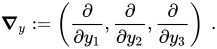
Define

$\boldsymbol{\nabla}_y := \left(\frac{\partial }{\partial y_1}, \frac{\partial }{\partial y_2}, \frac{\partial }{\partial y_3}\right)~.$

Then, for a vector field $\mathbf{v}(\mathbf{y})$ , using the chain rule we get

$\text{(10)} \qquad \boldsymbol{\nabla} \cdot \mathbf{v}(\mathbf{y}) = \cfrac{1}{\eta}~\boldsymbol{\nabla}_y \cdot\mathbf{v}(\mathbf{y}) ~;~~ \boldsymbol{\nabla} \times \mathbf{v}(\mathbf{y}) = \cfrac{1}{\eta}~\boldsymbol{\nabla}_y\times{\mathbf{v}(\mathbf{y})} ~.$

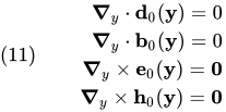
Using definitions (10) in (9) and collecting terms of order $1 / η$ gives

$\text{(11)} \qquad { \begin{align} \boldsymbol{\nabla}_y \cdot\mathbf{d}_0(\mathbf{y}) = 0 \\ \boldsymbol{\nabla}_y \cdot\mathbf{b}_0(\mathbf{y}) = 0 \\ \boldsymbol{\nabla}_y\times{\mathbf{e}_0(\mathbf{y})} = \boldsymbol{0} \\ \boldsymbol{\nabla}_y\times{\mathbf{h}_0(\mathbf{y})} = \boldsymbol{0} \end{align} }$

These are the solutions in the quasistatic limit. Also, from the constitutive equations

$\mathbf{d}_0(\mathbf{y}) = \epsilon(\mathbf{y})~\mathbf{e}_0(\mathbf{y}) ~;~~ \mathbf{b}_0(\mathbf{y}) = \mu(\mathbf{y})~\mathbf{h}_0(\mathbf{y}) ~.$

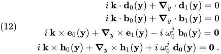
Similarly, collecting terms of order 1 from the expanded Maxwell's equations (9) we get

$\text{(12)} \qquad { \begin{align} i~\mathbf{k}\cdot\mathbf{d}_0(\mathbf{y}) + \boldsymbol{\nabla}_y \cdot\mathbf{d}_1(\mathbf{y}) = 0 \\ i~\mathbf{k}\cdot\mathbf{b}_0(\mathbf{y}) + \boldsymbol{\nabla}_y \cdot\mathbf{b}_1(\mathbf{y}) = 0 \\ i~\mathbf{k}\times\mathbf{e}_0(\mathbf{y}) + \boldsymbol{\nabla}_y\times{\mathbf{e}_1(\mathbf{y})} - i~\omega_0^j~\mathbf{b}_0(\mathbf{y}) = \boldsymbol{0} \\ i~\mathbf{k}\times\mathbf{h}_0(\mathbf{y}) + \boldsymbol{\nabla}_y\times{\mathbf{h}_1(\mathbf{y})} + i~\omega_0^j~\mathbf{d}_0(\mathbf{y}) = \boldsymbol{0} ~. \end{align} }$

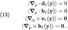
Since $\mathbf{d}_1(\mathbf{y}), \mathbf{b}_1(\mathbf{y}), \mathbf{e}_1(\mathbf{y}), \mathbf{h}_1(\mathbf{y})$ are periodic, this implies that

$\text{(13)} \qquad { \begin{align} \langle \boldsymbol{\nabla}_y \cdot\mathbf{d}_1(\mathbf{y})\rangle = 0 \\ \langle \boldsymbol{\nabla}_y \cdot\mathbf{b}_1(\mathbf{y})\rangle = 0 \\ \langle \boldsymbol{\nabla}_y \times{\mathbf{e}_1(\mathbf{y})}\rangle = \boldsymbol{0} \\ \langle \boldsymbol{\nabla}_y \times{\mathbf{h}_1(\mathbf{y})}\rangle = \boldsymbol{0} ~. \end{align} }$

where $\langle \bullet \rangle$ is the volume average over the unit cell. So a necessary condition that equations (12) have a solution is that

$\text{(14)} \qquad { \begin{align} i~\mathbf{k}\cdot\langle \mathbf{d}_0(\mathbf{y}) \rangle = 0 \\ i~\mathbf{k}\cdot\langle \mathbf{b}_0(\mathbf{y}) \rangle = 0 \\ i~\mathbf{k}\times\langle \mathbf{e}_0(\mathbf{y}) \rangle - i~\omega_0^j~\langle \mathbf{b}_0(\mathbf{y}) \rangle = \boldsymbol{0} \\ i~\mathbf{k}\times\langle \mathbf{h}_0(\mathbf{y}) \rangle + i~\omega_0^j~\langle \mathbf{d}_0(\mathbf{y}) \rangle = \boldsymbol{0} ~. \end{align} }$

Note that the second pair of (14) implies the first pair.

[edit] Footnotes

↑ The following discussion is based on Ashcroft76 (p. 133-139).
↑ We can see that the two operators commute by working out the operations. Thus,

$\mathcal{T}_R~\mathcal{L}~\begin{bmatrix}\mathbf{D} \\ \mathbf{B}\end{bmatrix} = \mathcal{T}_R~\begin{bmatrix} -i~\boldsymbol{\nabla} \times [\mu^{-1}(\mathbf{x})~\mathbf{B}(\mathbf{x})] \\ i~\boldsymbol{\nabla} \times [\epsilon^{-1}(\mathbf{x})~\mathbf{D}(\mathbf{x})] \end{bmatrix} = \begin{bmatrix} -i~\boldsymbol{\nabla} \times [\mu^{-1}(\mathbf{x}+\mathbf{R})~\mathbf{B}(\mathbf{x}+\mathbf{R})] \\ i~\boldsymbol{\nabla} \times [\epsilon^{-1}(\mathbf{x}+\mathbf{R})~\mathbf{D}(\mathbf{x}+\mathbf{R})] \end{bmatrix} = \mathcal{L}~\begin{bmatrix}\mathbf{D}(\mathbf{x}+\mathbf{R}) \\ \mathbf{B}(\mathbf{x}+\mathbf{R})\end{bmatrix} = \mathcal{L}~\mathcal{T}_R~\begin{bmatrix}\mathbf{D} \\ \mathbf{B}\end{bmatrix} ~.$
↑ We can see that the translation operator commutes by working out the operations. Thus,

$\mathcal{T}_R~\mathcal{T}_{R'}~ \begin{bmatrix} \mathbf{D}(\mathbf{x}) \\ \mathbf{B}(\mathbf{x}) \end{bmatrix} = \mathcal{T}_R~ \begin{bmatrix} \mathbf{D}(\mathbf{x}+\mathbf{R}') \\ \mathbf{B}(\mathbf{x}+\mathbf{R}') \end{bmatrix} = \begin{bmatrix} \mathbf{D}(\mathbf{x}+\mathbf{R}'+\mathbf{R}) \\ \mathbf{B}(\mathbf{x}+\mathbf{R}'+\mathbf{R}) \end{bmatrix} = \mathcal{T}_{R+R'}~ \begin{bmatrix} \mathbf{D}(\mathbf{x}) \\ \mathbf{B}(\mathbf{x}) \end{bmatrix} = \mathcal{T}_{R'}~ \begin{bmatrix} \mathbf{D}(\mathbf{x}+\mathbf{R}) \\ \mathbf{B}(\mathbf{x}+\mathbf{R})\end{bmatrix} = \mathcal{T}_{R'}~\mathcal{T}_{R}~ \begin{bmatrix}\mathbf{D}(\mathbf{x}) \\ \mathbf{B}(\mathbf{x})\end{bmatrix} ~.$
↑ The following discussion is based on Milton02

[edit] References

N. W. Ashcroft and N. D. Mermin. Solid State Physics. Saunders, New York, 1976.
G. W. Milton. Theory of Composites. Cambridge University Press, New York, 2002.

[0] The following discussion is based on Ashcroft76 (p. 133-139).

[1] We can see that the two operators commute by working out the operations. Thus,

$\mathcal{T}_R~\mathcal{L}~\begin{bmatrix}\mathbf{D} \\ \mathbf{B}\end{bmatrix} = \mathcal{T}_R~\begin{bmatrix} -i~\boldsymbol{\nabla} \times [\mu^{-1}(\mathbf{x})~\mathbf{B}(\mathbf{x})] \\ i~\boldsymbol{\nabla} \times [\epsilon^{-1}(\mathbf{x})~\mathbf{D}(\mathbf{x})] \end{bmatrix} = \begin{bmatrix} -i~\boldsymbol{\nabla} \times [\mu^{-1}(\mathbf{x}+\mathbf{R})~\mathbf{B}(\mathbf{x}+\mathbf{R})] \\ i~\boldsymbol{\nabla} \times [\epsilon^{-1}(\mathbf{x}+\mathbf{R})~\mathbf{D}(\mathbf{x}+\mathbf{R})] \end{bmatrix} = \mathcal{L}~\begin{bmatrix}\mathbf{D}(\mathbf{x}+\mathbf{R}) \\ \mathbf{B}(\mathbf{x}+\mathbf{R})\end{bmatrix} = \mathcal{L}~\mathcal{T}_R~\begin{bmatrix}\mathbf{D} \\ \mathbf{B}\end{bmatrix} ~.$

[2] We can see that the translation operator commutes by working out the operations. Thus,

$\mathcal{T}_R~\mathcal{T}_{R'}~ \begin{bmatrix} \mathbf{D}(\mathbf{x}) \\ \mathbf{B}(\mathbf{x}) \end{bmatrix} = \mathcal{T}_R~ \begin{bmatrix} \mathbf{D}(\mathbf{x}+\mathbf{R}') \\ \mathbf{B}(\mathbf{x}+\mathbf{R}') \end{bmatrix} = \begin{bmatrix} \mathbf{D}(\mathbf{x}+\mathbf{R}'+\mathbf{R}) \\ \mathbf{B}(\mathbf{x}+\mathbf{R}'+\mathbf{R}) \end{bmatrix} = \mathcal{T}_{R+R'}~ \begin{bmatrix} \mathbf{D}(\mathbf{x}) \\ \mathbf{B}(\mathbf{x}) \end{bmatrix} = \mathcal{T}_{R'}~ \begin{bmatrix} \mathbf{D}(\mathbf{x}+\mathbf{R}) \\ \mathbf{B}(\mathbf{x}+\mathbf{R})\end{bmatrix} = \mathcal{T}_{R'}~\mathcal{T}_{R}~ \begin{bmatrix}\mathbf{D}(\mathbf{x}) \\ \mathbf{B}(\mathbf{x})\end{bmatrix} ~.$

[3] The following discussion is based on Milton02

[1]

[2]

[3]

[4]

Waves in composites and metamaterials/Bloch waves and the quasistatic limit

From Wikiversity

Contents

[edit] Bloch Theorem

[edit] Quasistatic Limit

[edit] Footnotes

[edit] References

Views

Personal tools

Search

Navigation

Community

Toolbox