Report 4
For the series shown in the notes on p. 7-20
![{\displaystyle \ \sum _{j=0}^{n-2}[c_{j+2}(j+2)(j+1)+ac_{j+1}(j+1)+bc_{j}]x^{j}+ac_{n}nx^{n-1}+b[c_{n-1}x^{n-1}+c_{n}x^{n}]=\sum _{j=0}^{n}d_{j}x^{j}\ }](https://wikimedia.org/api/rest_v1/media/math/render/svg/855d121b62fb2319235f77fc88bf9e8d62e0f0ac)
Obtain the equations for the coefficients of  ,
,  ,
,  ,
,  ,
, 
Then, set up the coefficient matrix A for the general case with the coefficients obtained.
For j=0:
 (1)
(1)
For j=1:
 (2)
(2)
For j=2:
 (3)
(3)
For j=n-2:
![{\displaystyle \displaystyle [c_{n}(n)(n-1)+ac_{n-1}(n-1)+bc_{n-2}]=d_{n-2}}](https://wikimedia.org/api/rest_v1/media/math/render/svg/b823a41d459a00ba75e9ae89a049e1f8ae3c1ed6) (4)
(4)
For j=n-1:
 (5)
(5)
For j=n:
 (6)
(6)
Setting up the A matrix using equations (1)-(6):

Solved and uploaded by Joshua House
Proofread by David Herrick
Consider the L2-ODE-CC(5) p.7b-7 with sin x as excitation:


and with the initial conditions

Use the Taylor series for  in (1)p6-4 to reproduce the figure on p7-24
Let  be the particular soln corresponding to the excitating
  :
:

Let be the truncated Taylor series of sin x :

Let  be the overall soln for the L2-ODE-CC corresponding to (2)-(3) p.7-26 :

with the same initial conditions (3b)p.3-7.
Find the for n = 3, 5, 9; plot these solns for x in the interval [0,4π].
Use the particular soln in K 2011 p.82 Table 2.1 to find the exact overall soln y(x) and plot it in the above figure to compare with for n = 3, 5, 9.
To solve the non-homogeneous ODE we have to solve the homogeneous ODE and find any solution of  . Using the method of undetermined coefficients, specifically the basic rule, where r(x) is in one of the functions in the first column in Table 2.1 K 2011 p. 82 and choose the in the same line and determine its undetermined coefficients by substituting
  and its derivatives.
For an excitation 
n = 3

n = 5

n = 9

The term in  that will be used will be
For n = 3

For n = 5

For n = 9

The homogeneous solution for y will be in the form of

Plugging  into the original equation will give the following:
For n = 3

For n = 5


For n = 9


Equating the coefficients of  on both sides
For n = 3


Now plugging in the particular and homogeneous equation  and solving for the initial conditions.


This gives constant values of


For n = 3 Final solution is:

For n = 5
Equating the coefficients


Now plugging in the particular and homogeneous equation
and solving for the initial conditions.


This gives constant values of


For n = 5 the final solution is

For n = 9
Equating the coefficients


Now plugging in the particular and homogeneous equation
and solving for the initial conditions.


This gives constant values of


For n = 9 the final solution is


The table 2.1 from K 2011 p.82 illustrates that for the method of undetermined coefficients for an r(x) term in the form of:
r(x) = k sin(ωx)
Then the choice for would be:
K cos(ωx) + M sin(ωx)
The homogeneous solution for y will be in the form of

with roots of 2 and 1 derived from 
Plugging in the derivatives for the particular solution into the original equation gives:

where


Combining the particular and homogeneous solution of y gives the following:

Solving for the initial conditions where 


This gives the final solution:


From the figure it is barely discernible between this figure and the figure above it in part two. The final solution for y in part three is very similar if not approximately identical to the lower curve in the figure in part two.
This problem was solved and uploaded by Michael Wallace
Consider the L2-ODE-CC:
Where 
with initial conditions 
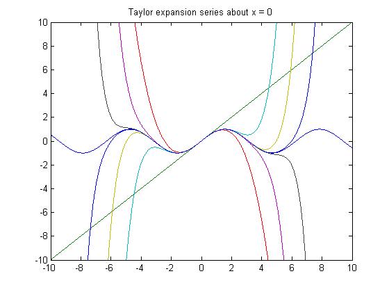
Develop  in Taylor series about x(hat) = 0 to reproduce the figure in the notes on p. 7-25.
Let be the truncated Taylor series with n terms -- which is also the highest degree of the Taylor (power) series -- of .
Find  for n = 4, 7, and 11 such that:

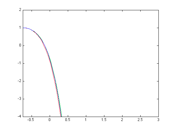
Plot for n = 4,7,11 for x in ![{\displaystyle \displaystyle \ [-{\frac {3}{4}},3]\ }](https://wikimedia.org/api/rest_v1/media/math/render/svg/283e3e8c951595edf73224c1f92ce252799076be)
Use the matlab command ODE45 to integrate numerically the same function with the same initial conditions to obtain  . Then plot in the same figure with
The formula to develop the Taylor Series about x(hat) = 0 is given by:

Using the function we get:

Plugging in 0, the first few terms become:

The pattern of this expression can be represented by the Taylor series:

First, the homogenous solution to the differential equation is given by:

Therefore, 
for is given by the truncated Taylor series of 4 terms:

Therefore, 

For this solution, with n = 4, the coefficient matrix is set up like:

Therefore, the matrix solution with n = 4, a = -3, and b = 2 is:

Solving by back substitution we get:


Plugging in the initial conditions we get:

for is given by the truncated Taylor series of 7 terms:

Therefore:


For this solution, with n = 7, the coefficient matrix is set up like:

Therefore, the matrix solution with n = 7, a = -3, and b = 2 is:

Solving by back substitution we get:

Since the homogeneous solution remains the same:

Plugging in the initial conditions we get:

The image below demonstrates the general matrix for n=11 and the matrix with values filled in:

for is given by the truncated Taylor series of 11 terms:

Therefore, 
Solving by back substitution we get:


Since the homogeneous solution remains the same:


Plugging in the initial conditions we get:


Matlab Code:
function yp = F(t,y)
yp = zeros(2,1);
yp(1) = y(2);
yp(2) = log(t+1) + 3*y(2)-2*y(1);
end
[t,y] = ode45('F',[-.75,3],[1,0]);
plot(x,y4,'g',x,y7,'r',x,y11,'y',t,y(:,1),'b')
axis([-0.75 3 -4 2])
Part 2 n=7 and n =11 were solved and uploaded by Cameron North.
Part 1 and Part 2 n = 4 was solved and uploaded by David Herrick
Find n sufficiently high so that  do not differ from the numerical solution by more than
  at
at 
Develop log(1+x) in Taylor series about  . Plot the results.
Find  for n=4,7,11, such that
  for x in [0.9,3] with the initial conditions found in Part 1. Plot the results.
Use the matlab command 'ode45' to integrate numerically (5) p.7b-7 with (1) p.7-28 and the initial conditions  to obtain the numerical solution for
  .
.
Plot in the same figure with 
With MATLAB, a program was used to iteratively add terms into the taylor series of  . Until the error between the exact answer and the series was less than ., more terms were added.

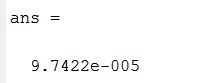
 for the error to be of a magnitude of . The error found:
9.7422e-005
for the error to be of a magnitude of . The error found:
9.7422e-005
With a very similar process for  .
.


 for the error to be of a magnitude of . The error found:
9.3967e-005
for the error to be of a magnitude of . The error found:
9.3967e-005
The formula to develop the Taylor Series about is given by:

Using the function for n=11 we get:


Plugging in x=1 up to n=4, and using the formula for developing the Taylor Series, we get  :
:
 ,
,
Then we do the same for n=7 terms to get  :
:

And finally for  :
:

Plotting the functions:
Matlab code:
x=-3:0.2:6;
y = log(1+x);
y4 = log(2) + (x-1)/2 - (x-1).^2/8 + (x-1).^3/24 - (x-1).^4/64;
y7 = log(2) + (x-1)/2 - (x-1).^2/8 + (x-1).^3/24 - (x-1).^4/64 + (x-1).^5/160 - (x-1).^6/384 + (x-1).^7/896;
y11 = log(2) + (x-1)/2 - (x-1).^2/8 + (x-1).^3/24 - (x-1).^4/64 + (x-1).^5/160 - (x-1).^6/384 + (x-1).^7/896 - (x-1).^8/2048 + (x-1).^9/4608 - (x-1).^(10)/10240 + (x-1).^(11)/22528;
plot(x,y, x,y4, x,y7, x,y11)
hleg1 = legend('log(1+x)','n=4','n=7','n=11');
Graph:
Convergence is in the domain [-1.5,4].
For n=4  is:
is:


 ,
,
Plugging the equations into the above ODE will give matrices like the following:

The unknown vector  can be solved by forward substitution,
with MATLAB to do the calculations:
can be solved by forward substitution,
with MATLAB to do the calculations:

Particular and general solution  ,
,  :
:


Then with the Initial Conditions,

For n=7 is:


The same process used when solving when n=4 is used to construct a matrix equation for n=7:

Using MATLAB to solve for the unknown vector :

Particular and general solutions  ,
,  :
:


With the initial conditions:

For n=11 is:


Creating another matrix system and solving for the unknown vector :


Particular and general solutions  ,
,  :
:


With initial conditions:

plot:
The initial condition equation is:

The initial conditions are:

To solve the problem, we first convert the 2nd order differential equation into two 1st order differential equations. The initial 2nd order then turns into these two equations:

Taking the derivatives, we find that:

with the new initial conditions as:

Now, we create a MATLAB function, "F", that will return a vector-valued function. We do this with the following function:
function yp=F(x,y)
yp=zeros(2,1);
yp(1)=y(2);
yp(2)=-2*y(1)-3*y(2)+log(1+x);
We now incorporate the function into a simple MATLAB program which will calculate the results:
EDU>> [x,y]=ode45('F',[0,5],[39,74]);
EDU>> plot(y(:,1),y(:,2))
This generates the following graph of :

Now we solve the initial value problem by hand to find y(x):
First, convert to the characteristic equation:


The excitation factor of ln(1+x) does not yield any useful value for  since the integral is nonelementary. Therefore, the final solution for y(x) with what is know is simply:


Graphing both solutions on the same graph yields the following:
MATLAB code: EDU>> z = 4*exp(x) + 25*exp(2*x)
plot(y(:,1),y(:,2),y(:,1),z)

Problem 1 was solved and uploaded by Joshua House 15:34, 13 March 2012 (UTC)
Problem 2 was solved by Mike Wallace
Problem 3 part 2 was solved by John North and parts 1 and 3 were solved by David Herrick
Problem 4 part 1 and part of part3 were solved and uploaded by Derik Bell, parts 2 and 3 were solved by Radina Dikova, and part 4 was solved by William Knapper


