Report 4
Intermediate Engineering Analysis
Section 7566
Team 11
Due date: March 14, 2012.
Obtain equations (2), (3), (n-2), (n-1), (n), and set up the matrix A as in (1) p.7-21
for the general case, with the matrix coefficients for rows 1, 2, 3, (n-2), (n-1), n, filled in,
as obtained from equations (1), (2), (3), (n-2), (n-1), (n).
As shown in p.7-21, the first equation is:
 (1) p.7-21
According to p.7-20, the general form of the series is:
![{\displaystyle \sum _{j=0}^{n-2}[c_{j+2}(j+2)(j+1)+ac_{j+1}+bc_{j}]x^{j}+ac_{n}nx^{n-1}+b[c_{n-1}x^{n-1}+c_{n}x^{n}]=\sum _{j=0}^{n}d_{j}x^{j}\!}](https://wikimedia.org/api/rest_v1/media/math/render/svg/6d5b39d8b5978e7e6059a343f46c4ebdf2cf61c6) (2) p. 7-20
(2) p. 7-20
From (2) p.7-20, we can obtain n+1 equations for n+1 unknown coefficients  .
.
After referring to p.7-22, it can be determined that the matrix to be set up is of the following form:

where the rows signify the coefficients  ,
and the columns signify
,
and the columns signify  .
.
Building the coefficient matrix as shown in p.7-22 of the class notes, we can begin to solve for the coefficients
as follows:
Equation associated with  :
:
j=0:  (1)
(1)
Equation associated with  :
:
j=1:  (2)
(2)
Equation associated with  :
:
j=2:  (3)
(3)
Equation associated with  :
:
j=n-2: ![{\displaystyle d_{n-2}=[c_{n}(n)(n-1)+ac_{n-1}(n-1)+bc_{n-2}]\!}](https://wikimedia.org/api/rest_v1/media/math/render/svg/a77c2db157f275bc2f747f87c340d4c18dfc5073) (n-2)
(n-2)
Equation associated with  :
:
j=n-1:  (n-1)
(n-1)
Equation associated with  :
:
j=n:  (n)
(n)
Using all of the above equations, (1), (2), (3), (n-2), (n-1), (n), we can then determine the A matrix to be:

Solved by Gonzalo Perez
Solved by Jonathan Sheider
Given: 
With initial conditions: 
Using the Taylor series for sin(x), reproduce the graph in the lecture notes p.7-24.
The Taylor series expansion for sin(x) that is plotted with n = 13 is as follows:

Using MatLab, the following Taylor series expansion was plotted and coded:

The plot created with n = 13 (i.e. 13 terms) is as follows:

Solved by Jonathan Sheider
Given: 
With initial conditions:
Letting  equal the truncated Taylor series of
  , i.e.
Find the overall solution  for
for  and plot these solutions on the interval from
 ![{\displaystyle [0,4\pi ]\!}](https://wikimedia.org/api/rest_v1/media/math/render/svg/419d1454d9668fee313b92eb4dde496859698a95)
First finding the homogenous solution to the ODE:
The characteristic equation:


Therefore, 
And the homogenous solution is:

Next the particular solution will be evaluated.
For n = 3:
The excitation is therefore: 
Therefore the particular solution has a form:

Differentiating:


Plugging these values into the ODE and equating them to the excitation:


To solve this, we will use an upper triangular matrix, and solve using Matlab. The matrix is as follows:

The answer is calculated in Matlab:

Therefore: 
The final solution is then found to be: 
Evaluating at the initial conditions, we have:


Solving this system of equations, we find:

Therefore the final solution is:

Plotting this equation in Matlab yields:

For n = 5:
The excitation is therefore: 
Therefore the particular solution has a form:

Differentiating:


Plugging these values into the ODE and equating them to the excitation, and then solving them by using a upper triangular matrix as before (just as in the n=3 example) in Matlab:

Therefore: 

The final solution is then found to be: 
Evaluating at the initial conditions, we have:


Solving this system of equations, we find:

Therefore the final solution is:

Plotting this equation in Matlab yields:
For n = 9:
The excitation is therefore: 
Therefore the particular solution has a form:


Differentiating:


Plugging these values into the ODE and equating them to the excitation, and then solving them by using an upper triangular matrix as before (just as in the n=3 example) in Matlab:
Therefore: 


The final solution is then found to be: 
Evaluating at the initial conditions, we have:


Solving this system of equations, we find:

Therefore the final solution is:


Plotting this equation in Matlab yields:
Note: On the interval from  to
to  , the resulting plots of the solutions, on such a large scale (note that the Y-axis is forced to be on the order of
  !) each plot looks almost exactly identical. It is not until you are able to zoom in a lot do you see the very slight change in the curve of each plot on this interval.
--Egm4313.s12.team11.sheider (talk) 01:09, 14 March 2012 (UTC)
Solved by Daniel Suh
Using the particular solution from Table 2.1 on Kreyszig, find the overall solution  , and plot it compared with for n = 3,5,9


Initial Conditions:  ,
, 
To find  ,
,


To find  ,
,
Using Table 2.1, we find that for ,


Plugging it back into the equation,


Solving for coefficients,


Solving with initial conditions,


Plotting in matlab yields:

As shown on the graph, the two plots are exactly the same.
Created by [Daniel Suh] 20:43, 13 March 2012 (UTC)
Solved by Francisco Arrieta
- Develop
 in Taylor Series about
  to reproduce the figure on page 7-25

For n=4:

For n=7:

For n=11:

For n=16:
-


Using MATLAB
--Egm4313.s12.team11.arrieta (talk) 00:44, 14 March 2012 (UTC)
Solved by: --Egm4313.s12.team11.vargas.aa (talk) 01:28, 14 March 2012 (UTC)
Given:
where 
With initial conditions: 
Find the overall solution for  and plot these solutions on the interval from
 ![{\displaystyle [-{\frac {3}{4}},3]\!}](https://wikimedia.org/api/rest_v1/media/math/render/svg/308e17971be2299355ca353c40d0f3ee8007b72a)
First we find the homogeneous solution to the ODE:
The characteristic equation is:
Then,
Therefore the homogeneous solution is:

Now to find the particulate solution
For n=4


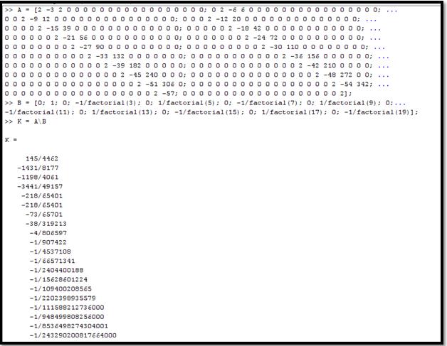
We can then use a matrix to organize the known coefficients:

Then, using MATLAB and the backlash operator we can solve for these unknowns:

Therefore

Superposing the homogeneous and particulate solution we get

Differentiating:
 Evaluating at the initial conditions:


We obtain:


Finally we have:

For n=7

We can then use a matrix to organize the known coefficients:

Then, using MATLAB and the backlash operator we can solve for these unknowns:

Therefore

Superposing the homogeneous and particulate solution we get

Differentiating:
 Evaluating at the initial conditions:


We obtain:


Finally

For n=11
We can then use a matrix to organize the known coefficients:


Then, using MATLAB and the backlash operator we can solve for these unknowns:

Therefore


Superposing the homogeneous and particulate solution we get


Differentiating:


Evaluating at the initial conditions:


We obtain:


Finally

Plot for part 2 and part 3. Please note that because of the broad scale, it is almost impossible to distinguish between the graphs for n=4,7,11 nad the ODE45 operator. Only when zoomed in is there any noticeable difference

Find n sufficiently high so that  do not differ from the numerical solution by more than
  at
at 
Using a program in MATLAB that iteratively added terms onto the taylor series of  , terms were added until the error between the exact answer and the series was less than .

It was found after trial and error that  for the error to be of a magnitude of . This error found was
9.7422e-005
for the error to be of a magnitude of . This error found was
9.7422e-005
Similarly, for  .
.

It was found after trial and error that  for the error to be of a magnitude of . This error found was
9.3967e-005
for the error to be of a magnitude of . This error found was
9.3967e-005
Develop in Taylor series about  for
for  and plot these truncated series vs. the exact function.
What is now the domain of convergence by observation?
A MATLAB program was created, which calculated the Taylor series of each n value, along with the exact function, then plotted these together to show the comparison of all the series.
Below is the Taylor series for  expanded at .


It can be seen by observation that the domain of convergence has shifted to the right one unit.
--egm4313.s12.team11.gooding (talk) 03:48, 14 March 2012 (UTC)
Solved by Luca Imponenti
Find , for such that:

for  in
in ![{\displaystyle [0.9,3]\!}](https://wikimedia.org/api/rest_v1/media/math/render/svg/bb2c515c8c74080e5a7916ac7bd889dc9164916e) with the initial conditions found.
with the initial conditions found.
Plot for for in .
The homogeneous case is shown below:

This equation has the following roots:

Which gives yields the homogeneous solution
Using the taylor series approximation from earlier with  we have

We know the particular solution,  , ve will have this form:

taking the derivatives of this solution

and

Plugging the above equations into the original ODE yields the following matrix equation:

The unknown vector  can be easily solved by forward substitution,the following values were calculated in matlab:

So the particular solution  is
is

We can now find the general solution for n=4,  .
.


Solving using the initial conditions yields;

Using the taylor series approximation from earlier with  we have

In a similar fashion we construct a matrix equation for n=7:

Solving:

So the particular solution  is
is

We can now find the general solution for n=7,  .
.


Solving using our initial conditions yields


Using the taylor series approximation from earlier with  we have


Finally, we write out the matrix equation for n=11:


Solving the system in matlab:


So the particular solution  is
is


We can now find the general solution for n=11,  .
.


Solving using our initial conditions yields


 shown in red
 shown in blue
 shown in green

Solved by Luca Imponenti
Use the matlab command ode45 to integrate numerically with 
and the initial conditions from Part 3 to obtain the numerical solution for y(x).
Plot y(x) in the same figure as above.
The numerical solution calculated using the matlab ode45 command is shown below:
 ans =
   0.2788
   0.2854
   0.2923
   0.2997
   0.3074
   0.3229
   0.3401
   0.3592
   0.3804
   0.4040
   0.4302
   0.4595
   0.4921
   0.5285
   0.5691
   0.6145
   0.6651
   0.7218
   0.7850
   0.8557
   0.9346
   1.0228
   1.1213
   1.2313
   1.3542
   1.4914
   1.6445
   1.8155
   2.0063
   2.2193
   2.4569
   2.7219
   3.0175
   3.3471
   3.7146
   4.1243
   4.5809
   5.0898
   5.6568
   6.2885
   6.9921
   7.3442
   7.7142
   8.1032
   8.5119
Plotting the aboved vector of y-values,along with the results from earlier yields the following graph:

where the answer calculated in matlab is shown in yellow.
Egm4313.s12.team11.imponenti (talk) 08:04, 14 March 2012 (UTC)


