Nonlinear finite elements/Kinematics - polar decomposition

Polar decomposition

The w:Polar decomposition theorem states that any second order tensor whose determinant is positive can be decomposed uniquely into a symmetric part and an orthogonal part.

In continuum mechanics, the deformation gradient ${\boldsymbol {F}}$ is such a tensor because $\det(\mathbf {F} )>0$. Therefore we can write

${\boldsymbol {F}}={\boldsymbol {R}}\cdot {\boldsymbol {U}}={\boldsymbol {V}}\cdot {\boldsymbol {R}}$

where ${\boldsymbol {R}}$ is an orthogonal tensor (${\boldsymbol {R}}\cdot {\boldsymbol {R}}^{T}={\boldsymbol {\mathit {1}}}$) and ${\boldsymbol {U}},{\boldsymbol {V}}$ are symmetric tensors (${\boldsymbol {U}}={\boldsymbol {U}}^{T}$ and ${\boldsymbol {V}}={\boldsymbol {V}}^{T}$) called the right stretch tensor and the left stretch tensor, respectively. This decomposition is called the polar decomposition of ${\boldsymbol {F}}$.

Recall that the right Cauchy-Green deformation tensor is defined as

${\boldsymbol {C}}={\boldsymbol {F}}^{T}\cdot {\boldsymbol {F}}$

Clearly this is a symmetric tensor. From the polar decomposition of ${\boldsymbol {F}}$ we have

${\boldsymbol {C}}={\boldsymbol {U}}^{T}\cdot {\boldsymbol {R}}^{T}\cdot {\boldsymbol {R}}\cdot {\boldsymbol {U}}={\boldsymbol {U}}\cdot {\boldsymbol {U}}={\boldsymbol {U}}^{2}$

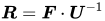
If you know ${\boldsymbol {C}}$ then you can calculate ${\boldsymbol {U}}$ and hence ${\boldsymbol {R}}$ using ${\boldsymbol {R}}={\boldsymbol {F}}\cdot {\boldsymbol {U}}^{-1}$.

How do you find the square root of a tensor?

If you want to find ${\boldsymbol {U}}$ given ${\boldsymbol {C}}$ you will need to take the square root of ${\boldsymbol {C}}$. How does one do that?

We use what is called the spectral decomposition or eigenprojection of ${\boldsymbol {C}}$. The spectral decomposition involves expressing ${\boldsymbol {C}}$ in terms of its eigenvalues and eigenvectors. The tensor product of the eigenvectors acts as a basis while the eigenvalues give the magnitude of the projection.

Thus,

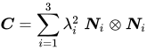
${\boldsymbol {C}}=\sum _{i=1}^{3}\lambda _{i}^{2}~{\boldsymbol {N}}_{i}\otimes {\boldsymbol {N}}_{i}$

where $\lambda _{i}^{2}$ are the principal values (eigenvalues) of ${\boldsymbol {C}}$ and ${\boldsymbol {N}}_{i}$ are the principal directions (eigenvectors) of ${\boldsymbol {C}}$.

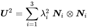
Therefore,

${\boldsymbol {U}}^{2}=\sum _{i=1}^{3}\lambda _{i}^{2}~{\boldsymbol {N}}_{i}\otimes {\boldsymbol {N}}_{i}$

Since the basis does not change, we then have

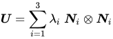
${\boldsymbol {U}}=\sum _{i=1}^{3}\lambda _{i}~{\boldsymbol {N}}_{i}\otimes {\boldsymbol {N}}_{i}$

Therefore the $\lambda _{i}$ can be interpreted as principal stretches and the vectors ${\boldsymbol {N}}_{i}$ are the directions of the principal stretches.

Exercise:

If

${\boldsymbol {U}}=\sum _{i=1}^{3}\lambda _{i}~{\boldsymbol {N}}_{i}\otimes {\boldsymbol {N}}_{i}$

show that

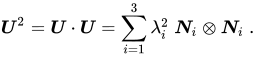
${\boldsymbol {U}}^{2}={\boldsymbol {U}}\cdot {\boldsymbol {U}}=\sum _{i=1}^{3}\lambda _{i}^{2}~{\boldsymbol {N}}_{i}\otimes {\boldsymbol {N}}_{i}~.$

Example of polar decomposition

Let us assume that the motion is given by

${\begin{aligned}x_{1}&={\cfrac {1}{4}}\left[4~X_{1}+(9-3~X_{1}-5~X_{2}-X_{1}~X_{2})~t\right]\\x_{2}&=X_{2}+(4+2~X_{1})~t\end{aligned}}$

The adjacent figure shows how a unit square subjected to this motion evolves over time.

An example of a motion.

Deformation gradient

The deformation gradient is given by

${\boldsymbol {F}}={\frac {\partial \mathbf {x} }{\partial {\boldsymbol {X}}}}\quad \implies \quad F_{ij}={\frac {\partial x_{i}}{\partial X_{j}}}$

Therefore

${\begin{aligned}F_{11}&={\frac {\partial x_{1}}{\partial X_{1}}}={\cfrac {1}{4}}\left[4+(-3-X_{2})~t\right]\\F_{12}&={\frac {\partial x_{1}}{\partial X_{2}}}={\cfrac {1}{4}}\left[(-5-X_{1})~t\right]\\F_{21}&={\frac {\partial x_{2}}{\partial X_{1}}}=2~t\\F_{22}&={\frac {\partial x_{2}}{\partial X_{2}}}=1\end{aligned}}$

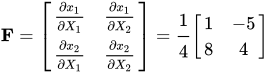
At $t=1$ at the position ${\boldsymbol {X}}=(0,0)$ we have

$\mathbf {F} ={\begin{bmatrix}{\frac {\partial x_{1}}{\partial X_{1}}}&{\frac {\partial x_{1}}{\partial X_{2}}}\\{\frac {\partial x_{2}}{\partial X_{1}}}&{\frac {\partial x_{2}}{\partial X_{2}}}\end{bmatrix}}={\cfrac {1}{4}}{\begin{bmatrix}1&-5\\8&4\end{bmatrix}}$

You can calculate the deformation gradient at other points in a similar manner.

Right Cauchy-Green deformation tensor

We have

${\boldsymbol {C}}={\boldsymbol {F}}^{T}\cdot {\boldsymbol {F}}$

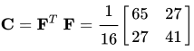
Therefore,

$\mathbf {C} =\mathbf {F} ^{T}~\mathbf {F} ={\cfrac {1}{16}}{\begin{bmatrix}65&27\\27&41\end{bmatrix}}$

To compute ${\boldsymbol {U}}$ we have to find the eigenvalues and eigenvectors of ${\boldsymbol {C}}$. The eigenvalue problem is

$(\mathbf {C} -\lambda ^{2}~\mathbf {I} )\mathbf {N} =\mathbf {0}$

where

$\mathbf {I} ={\begin{bmatrix}1&0\\0&1\end{bmatrix}}$

To find the eigenvalues we solve the characteristic equation

$\det(\mathbf {C} -\lambda ^{2}~\mathbf {I} )=0$

Plugging in the numbers, we get

$\det {\begin{bmatrix}{\cfrac {65}{16}}-\lambda ^{2}&{\cfrac {27}{16}}\\{\cfrac {27}{16}}&{\cfrac {41}{16}}-\lambda ^{2}\end{bmatrix}}=0$

or

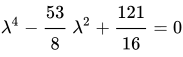
$\lambda ^{4}-{\cfrac {53}{8}}~\lambda ^{2}+{\cfrac {121}{16}}=0$

This equation has two solutions

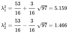
${\begin{aligned}\lambda _{1}^{2}&={\cfrac {53}{16}}+{\cfrac {3}{16}}~{\sqrt {97}}=5.159\\\lambda _{2}^{2}&={\cfrac {53}{16}}-{\cfrac {3}{16}}~{\sqrt {97}}=1.466\end{aligned}}$

Taking the square roots we get the values of the principal stretches

$\lambda _{1}=2.2714\qquad \lambda _{2}=1.2107$

To compute the eigenvectors we plug into the eigenvalues into the eigenvalue problem to get

$\left\{{\begin{bmatrix}65&27\\27&41\end{bmatrix}}-\lambda _{1}^{2}~{\begin{bmatrix}1&0\\0&1\end{bmatrix}}\right\}~{\begin{bmatrix}N_{1}^{(1)}\\N_{2}^{(1)}\end{bmatrix}}={\begin{bmatrix}0\\0\end{bmatrix}}$

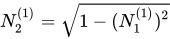
Because this system of equations is not linearly independent, we need another equation to solve this system of equations for $N_{1}^{(1)}$ and $N_{2}^{(1)}$. This problem is eliminated by using the following equation (which implies that $\mathbf {N}$ is a unit vector)

$N_{2}^{(1)}={\sqrt {1-(N_{1}^{(1)})^{2}}}$

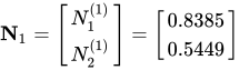
Solving, we get

$\mathbf {N} _{1}={\begin{bmatrix}N_{1}^{(1)}\\N_{2}^{(1)}\end{bmatrix}}={\begin{bmatrix}0.8385\\0.5449\end{bmatrix}}$

We can do the same thing for the other eigenvector $\mathbf {N} _{2}$ to get

$\mathbf {N} _{2}={\begin{bmatrix}N_{1}^{(2)}\\N_{2}^{(2)}\end{bmatrix}}={\begin{bmatrix}-0.5449\\0.8385\end{bmatrix}}$

Therefore,

${\boldsymbol {N}}_{1}\otimes {\boldsymbol {N}}_{1}=\mathbf {N} _{1}~\mathbf {N} _{1}^{T}={\begin{bmatrix}0.8385\\0.5449\end{bmatrix}}{\begin{bmatrix}0.8385&0.5449\end{bmatrix}}={\begin{bmatrix}0.7031&0.4569\\0.4569&0.2969\end{bmatrix}}$

and

${\boldsymbol {N}}_{2}\otimes {\boldsymbol {N}}_{2}=\mathbf {N} _{2}~\mathbf {N} _{2}^{T}={\begin{bmatrix}-0.5449\\0.8385\end{bmatrix}}{\begin{bmatrix}-0.5449&0.8385\end{bmatrix}}={\begin{bmatrix}0.2969&-0.4569\\-0.4569&0.7031\end{bmatrix}}$

Therefore,

${\boldsymbol {C}}=\lambda _{1}^{2}~{\boldsymbol {N}}_{1}\otimes {\boldsymbol {N}}_{1}+\lambda _{2}^{2}~{\boldsymbol {N}}_{2}\otimes {\boldsymbol {N}}_{2}\quad \implies \quad \mathbf {C} =5.159~{\begin{bmatrix}0.7031&0.4569\\0.4569&0.2969\end{bmatrix}}+1.466~{\begin{bmatrix}0.2969&-0.4569\\-0.4569&0.7031\end{bmatrix}}$

We usually don't see any problem to calculate ${\boldsymbol {C}}$ at this point and go straight to the right stretch tensor.

Right stretch

The right stretch tensor ${\boldsymbol {U}}$ is given by

${\boldsymbol {U}}=\lambda _{1}~{\boldsymbol {N}}_{1}\otimes {\boldsymbol {N}}_{1}+\lambda _{2}~{\boldsymbol {N}}_{2}\otimes {\boldsymbol {N}}_{2}\quad \implies \quad \mathbf {U} =2.2714~{\begin{bmatrix}0.7031&0.4569\\0.4569&0.2969\end{bmatrix}}+1.2107~{\begin{bmatrix}0.2969&-0.4569\\-0.4569&0.7031\end{bmatrix}}$

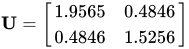
or

$\mathbf {U} ={\begin{bmatrix}1.9565&0.4846\\0.4846&1.5256\end{bmatrix}}$

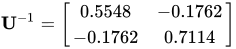
We can invert this matrix to get

$\mathbf {U} ^{-1}={\begin{bmatrix}0.5548&-0.1762\\-0.1762&0.7114\end{bmatrix}}$

Rotation

We can now find the rotation matrix by using th relation

${\boldsymbol {R}}={\boldsymbol {F}}\cdot {\boldsymbol {U}}^{-1}$

In matrix form,

$\mathbf {R} ={\cfrac {1}{4}}{\begin{bmatrix}1&-5\\8&4\end{bmatrix}}{\begin{bmatrix}0.5548&-0.1762\\-0.1762&0.7114\end{bmatrix}}={\begin{bmatrix}0.3590&-0.9334\\0.9334&0.3590\end{bmatrix}}$

You can check whether this matrix is orthogonal by seeing whether $\mathbf {R} ~\mathbf {R} ^{T}=\mathbf {R} ^{T}~\mathbf {R} =\mathbf {I}$.

You thus get the polar decomposition of ${\boldsymbol {F}}$. In an actual calculation you have to be careful about floating point errors. Otherwise you might not get a matrix that is orthogonal.

← Kinematics

Nonlinear finite elements

Kinematics - spectral decomposition →