Hilbert Book Model Project/Quaternionic Field Equations

HansVanLeunen respectfully asks that people use the discussion page, their talk page or email them, rather than contribute to this page at this time. This page might be under construction, controversial, used currently as part of a brick and mortar class by a teacher, or document an ongoing research project. Please RESPECT their wishes by not editing this page.

Quaternionic Field Equations

This page is currently being adapted by User:HansVanLeunen

Introduction

Maxwell equations apply the three-dimensional nabla operator in combination with a time derivative that applies coordinate time. The Maxwell equations derive from results of experiments. For that reason, those equations contain physical units.

In this treatment, the quaternionic partial differential equations apply the quaternionic nabla. The equations do not derive from the results of experiments. Instead, the formulas apply the fact that the quaternionic nabla behaves as a quaternionic multiplying operator. The corresponding formulas do not contain physical units. This approach generates essential differences between Maxwell field equations and quaternionic partial differential equations.

The quaternionic partial differential equations form a complete and self-consistent set. They use the properties of the three-dimensional spatial nabla. The corresponding formulas are taken from Bo Thidé's EMTF book., section Appendix F4. Another online resource is Vector_calculus_identities.

The quaternionic partial differential equations do not change the data format. The format of the information that the field transmits to observers, which the field embeds is affected by the information transfer. Instead of the Euclidean storage format, which governs at the location of the observed event, the observers perceive a spacetime format, which features a Minkowski signature. The Lorentz transform describes the format conversion.

Maxwell equations use coordinate time, where quaternionic differential equations use proper time.

Regarding quaternions, the norm of the quaternion plays the role of coordinate time. These time values apply not in their absolute versions. Thus, only time intervals apply.

Hilbert spaces can only cope with number systems that are division rings. In a division ring, all non-zero members own a unique inverse.

Only three suitable division rings exist. These are the real numbers, the complex numbers, and the quaternions.

Thus dynamic geometric data that are characterized by a Minkowski signature must first be dismantled into real numbers before they can serve in a Hilbert space.

Quaternions can store and retrieve without dismantling.

Quantum physicists use Hilbert spaces for the modeling of their theory. However, most quantum physicists apply complex number based Hilbert spaces.

Quaternionic quantum mechanics appears to represent a natural choice.

Format conversion

A read-only repository in the form of the combination of a quaternionic infinite dimensional separable Hilbert space and its non-separable companion stores the dynamic geometric data that constitute the observed event in a Euclidean format in the form of combinations of a timestamp and a three-dimensional spatial location. Quaternions act as storage containers. A private timestamp and a spatial location characterize the observer. The observer can only access storage locations whose timestamp predates his own timestamp. A continuum transfers this information to the observer. The speed of information transfer of the continuum is fixed. Therefore, the information transfer affects the format of the information that the observer perceives. A non-zero speed difference between observed event and observer will contract observed lengths will dilate durations. The Lorentz transform is a hyperbolic transform that describes the format conversion.

Quaternionic differential calculus describes the interaction between discrete objects and the continuum at the location where events occur. Converting the results of this calculus by the Lorentz transform will describe the information that the observers perceive. Observers perceive in spacetime format. This format features a Minkowski signature. The Lorentz transform converts from the Euclidean storage format at the situation of the observed event to the perceived spacetime format.

Storage model

In this model, the instant of storage of the event data is irrelevant as long as it precedes the stored time stamp. Thus the model can store all data at an instant, which precedes all stored timestamp values. This impersonates the model as a creator of the universe in which the observable events and the observers exist.

The repository merges Hilbert space operator technology with quaternionic function theory and quaternionic differential and integral calculus. The separable Hilbert space typically stores the discrete quaternionic data. These can occur as spurious data, as coherent swarms or as ordered distributions. Coordinate systems can order dense coherent swarms, which then become ordered distributions. Location density distributions can describe these ordered swarms. The non-separable Hilbert space embeds the separable Hilbert space, and in this way, the data sets become part of the non-separable Hilbert space. The non-separable Hilbert space stores continuums. In the non-separable Hilbert space, quaternionic functions describe continuums. The coherent swarms can embed in a continuum. The embedding process involves a convolution of the location density distribution of the coherent swarm with the Green's function of the continuum. Differential equations describe the behavior of the continuums. In this page, we only consider continuums that mostly continuous quaternionic functions can describe.

Fields

In the Hilbert Book Model fields are eigenspaces of operators that reside in the non-separable Hilbert space. Continuous or mostly continuous functions define these operators and apart from some discrepant regions their eigenspaces are continuums. These regions might reduce to single discrepant poinlike artefacts. The parameter space of these functions are constituted by quaternionic number systems. Consequently the real number valued coefficients of these parameters are mutually independent and the differential change can be expressed in terms of a linear combination of partial differentials. Now the total differential change ${\textstyle df}$ of field ${\textstyle f}$ equals

$df={\frac {\partial {f}}{\partial {\tau }}}d\tau +{\frac {\partial {f}}{\partial {x}}}{\vec {i}}dx+{\frac {\partial {f}}{\partial {y}}}{\vec {j}}dy+{\frac {\partial {f}}{\partial {z}}}{\vec {k}}dz$

(1)

In this equation, the partial differentials ${\textstyle {\frac {\partial {f}}{\partial {\tau }}},{\frac {\partial {f}}{\partial {x}}},{\frac {\partial {f}}{\partial {y}}},{\frac {\partial {f}}{\partial {z}}}}$ are quaternions.

The quaternionic nabla ${\textstyle \nabla }$ assumes the special condition that partial differentials direct along the axes of the Cartesian coordinate system. Thus

$\nabla =\sum _{i=1}^{n}{\vec {e}}_{i}{\partial \over \partial x_{i}}={\frac {\partial {}}{\partial {\tau }}}+{\vec {i}}{\frac {\partial {}}{\partial {x}}}+{\vec {j}}{\frac {\partial {}}{\partial {y}}}+{\vec {k}}{\frac {\partial {}}{\partial {z}}}$

(2)

The Hilbert Book Model assumes that the quaternionic fields are moderately changing, such that only first and second order partial differential equations describe the model. These equations can describe fields of which the continuity gets disrupted by pointlike artefacts. Warps, clamps and Green's functions describe such disruptions.

Generalized field equations

Generalized field equations hold for all basic fields. Generalized field equations fit best in a quaternionic setting.

Quaternions consist of a real number valued scalar part and a three-dimensional spatial vector that represents the imaginary part.

The multiplication rule of quaternions indicates that several independent parts constitute the product.

In this comment, we use a suffix ${\textstyle _{r}}$ to indicate the scalar real part of a quaternion, and we use ${\textstyle {\vec {a}}}$ to indicate the imaginary vector part of quaternion ${\textstyle a}$.

$c=c_{r}+{\vec {c}}=ab=(a_{r}+{\vec {a}})(b_{r}+{\vec {b}})=a_{r}b_{r}-\langle {\vec {a}},{\vec {b}}\rangle +a_{r}{\vec {b}}+{\vec {a}}b_{r}{\color {Red}\pm }{\vec {a}}\times {\vec {b}}$

(3)

The ${\textstyle {\color {Red}\pm }}$ in equation (3) indicates that quaternions exist in right-handed and left-handed versions.

The formula can be used to check the completeness of a set of equations that follow from the application of the product rule.

The quaternionic conjugate of a is ${\textstyle a^{*}=a_{r}-{\vec {a}}}$ From the product rule follows the formula for the norm ${\textstyle |a|}$ of quaternion ${\textstyle a}$.

$|a|^{2}=aa^{*}=(a_{r}+{\vec {a}})(a_{r}-{\vec {a}})=a_{r}a_{r}+\langle {\vec {a}},{\vec {a}}\rangle$

(4)

We define the quaternionic nabla as ${\textstyle \nabla =\left\{{\partial \over \partial \tau },{\partial \over \partial x},{\partial \over \partial y},{\partial \over \partial z}\right\}=\nabla _{r}+{\vec {\nabla }};\quad \nabla _{r}={\partial \over \partial \tau };\quad {\vec {\nabla }}=\left\{{\partial \over \partial x},{\partial \over \partial y},{\partial \over \partial z}\right\}}$.

The quaternionic nabla ${\textstyle \nabla }$ acts like a multiplying operator. The (partial) differential ${\textstyle \nabla \psi }$ represents the full first-order change of field ${\textstyle \psi }$. We assume that ${\textstyle \varphi =\nabla \psi }$ exists in an enclosed region of the domain of ${\textstyle \psi }$.

First order partial differential equation

$\varphi =\varphi _{r}+{\vec {\varphi }}=\nabla \psi =(\nabla _{r}+{\vec {\nabla }})(\psi _{r}+{\vec {\psi }})=\nabla _{r}\psi _{r}-\langle {\vec {\nabla }},{\vec {\psi }}\rangle +\nabla _{r}{\vec {\psi }}+{\vec {\nabla }}\psi _{r}{\color {Red}\pm }{\vec {\nabla }}\times {\vec {\psi }}$

(5)

The equation is a quaternionic first order partial differential equation.

The five terms on the right side show the components that constitute the full first-order change.

They represent subfields of field $\varphi$, and often they get special names and symbols.

Subfields

${\vec {\nabla }}\psi _{r}$ is the gradient of $\psi _{r}$

$\langle {\vec {\nabla }},{\vec {\psi }}\rangle$ is the divergence of ${\vec {\psi }}$.

${\vec {\nabla }}\times {\vec {\psi }}$ is the curl of ${\vec {\psi }}$

$\varphi _{r}=\nabla _{r}\psi _{r}-\langle {\vec {\nabla }},{\vec {\psi }}\rangle$

(6)

(Equation (6) has no equivalent in Maxwell's equations! Instead $\varphi _{r}=\nabla _{r}\psi _{r}-\langle {\vec {\nabla }},{\vec {\psi }}\rangle$ is used as a gauge )

${\vec {\varphi }}=\nabla _{r}{\vec {\psi }}+{\vec {\nabla }}\psi _{r}\pm {\vec {\nabla }}\times {\vec {\psi }}=\mp {\vec {B}}-{\vec {E}}$

(7)

${\vec {E}}\ {\overset {\underset {\mathrm {def} }{}}{=}}\ -\nabla _{r}{\vec {\psi }}-{\vec {\nabla }}\psi _{r}$

(8)

${\vec {B}}\ {\overset {\underset {\mathrm {def} }{}}{=}}\ {\vec {\nabla }}\times {\vec {\psi }}$

(9)

${\vec {J}}\ {\overset {\underset {\mathrm {def} }{}}{=}}\ {\vec {\nabla }}\times {\vec {B}}-\nabla _{r}{\vec {E}}$

(10)

Interpretation of terms

By replacing the nabla by a normalized direction in which change takes place, the vector terms in the first order partial differential equation get a particular interpretation, which will be used in the integral equations.

${\vec {\nabla }}\psi ={\vec {\nabla }}(\psi _{r}+{\vec {\psi }})=-\langle {\vec {\nabla }},{\vec {\psi }}\rangle +{\vec {\nabla }}\psi _{r}\pm {\vec {\nabla }}\times {\vec {\psi }}\Longleftrightarrow {\vec {n}}\psi ={\vec {n}}(\psi _{r}+{\vec {\psi }})=-\langle {\vec {n}},{\vec {\psi }}\rangle +\nabla _{r}{\vec {\psi }}+{\vec {n}}\psi _{r}\pm {\vec {n}}\times {\vec {\psi }}$

(11)

Properties of the spatial nabla operator

The nabla product is not associative. Thus

$\nabla (\nabla ^{*}\psi )=\nabla ^{*}(\nabla \psi )=(\nabla _{r}\nabla _{r}+\langle {\vec {\nabla }},{\vec {\nabla }}\rangle )\psi \neq (\nabla \nabla ^{*})\psi =(\nabla ^{*}\nabla )\psi =(\nabla _{r}\nabla _{r}+{\vec {\nabla }}{\vec {\nabla }})\psi =(\nabla _{r}\nabla _{r}-\langle {\vec {\nabla }},{\vec {\nabla }}\rangle \pm {\vec {\nabla }}\times {\vec {\nabla }})\psi$

The quaternionic nabla ${\textstyle \nabla }$ and the spatial nabla ${\textstyle {\vec {\nabla }}}$ behave in a complicated way. A special page is devoted to these nabla operators.

Second order partial differential equations

We start with the quaternionic equivalent of the Maxwell-Faraday equation.

$\nabla _{r}{\vec {B}}={\vec {\nabla }}\times (\nabla _{r}{\vec {\psi }})=-{\vec {\nabla }}\times {\vec {E}}$

(12)

Two interesting second order quaternionic partial differential equations exist.

$\zeta =(\nabla _{r}\nabla _{r}-\langle {\vec {\nabla }},{\vec {\nabla }}\rangle )\psi$

(13)

This is the quaternionic equivalent of the wave equation. It offers waves as part of the solutions of the homogeneous equation.

$\chi =\nabla ^{*}\varphi =\nabla ^{*}\nabla \psi =\nabla \nabla ^{*}\psi =(\nabla _{r}-{\vec {\nabla }})(\varphi _{r}+{\vec {\varphi }})=(\nabla _{r}+{\vec {\nabla }})(\nabla _{r}-{\vec {\nabla }})(\psi _{r}+{\vec {\psi }})=(\nabla _{r}\nabla _{r}+\langle {\vec {\nabla }},{\vec {\nabla }}\rangle )\psi$

(14)

This equation can be split into two first order partial wave equations $\chi =\nabla ^{*}\varphi$ and $\varphi =\nabla \psi$.

This equation does not offer waves as part of the solutions of the homogeneous equation.

Differential operators

$D=(\nabla _{r}\nabla _{r}-\langle {\vec {\nabla }},{\vec {\nabla }}\rangle )$

(15)

This is the quaternionic equivalent of d'Alembert's operator.

$\boxdot =(\nabla _{r}\nabla _{r}+\langle {\vec {\nabla }},{\vec {\nabla }}\rangle )$

(16)

This operator does not yet have a known name.

Operator $\langle {\vec {\nabla }},{\vec {\nabla }}\rangle$ represents the main part of the Poisson equation. Together with $\nabla _{r}\nabla _{r}$ this operator configures the above operators.

As is shown above, $\boxdot$ can be derived from the nabla operator. That cannot be said from the $D$ operator.

Wave equation from Maxwell equations

Gauge equations must extend Maxwell equations to derive the second order partial wave equation.

Solutions

The quaternionic second order partial wave equations offer a series of interesting solution that play an important role in the Hilbert Book Model. A special page is dedicated to these solutions.

Poisson equation and Green's function

The Poisson equation

$\phi =\langle {\vec {\nabla }},{\vec {\nabla }}\rangle \psi$

(17)

describes how the field reacts with its Green’s function $G$ on a point-like trigger.

$G({\vec {q}}-{\vec {c}})=1/|{\vec {q}}-{\vec {c}}|$

(18)

Passage through a surface and balance equations

Like Maxwell's equations, the quaternionic partial differential equations relate to surface-volume integrals. The differential equations are continuity equations and the integral equations represent balance equations. The Extended Stokes Theorem page treats the case that the encapsulated domain contains multiple parameter spaces.

The curl can be defined as

$({\vec {\nabla }}\times {\vec {\psi }})\cdot {\vec {n}}\ {\overset {\underset {\mathrm {def} }{}}{=}}\lim _{A\to 0}\left({\frac {1}{|A|}}\oint _{C}{\vec {\psi }}\cdot d{\vec {r}}\right)$

With respect to a local part of a closed boundary that is oriented perpendicular to vector 𝙣 the partial differentials relate as

${\vec {\nabla }}\psi ={\vec {\nabla }}(\psi _{r}+{\vec {\psi }})=-\langle {\vec {\nabla }},{\vec {\psi }}\rangle +{\vec {\nabla }}\psi _{r}\pm {\vec {\nabla }}\times {\vec {\psi }}\Longleftrightarrow {\vec {n}}\psi ={\vec {n}}(\psi _{r}+{\vec {\psi }})=-\langle {\vec {n}},{\vec {\psi }}\rangle +\nabla _{r}{\vec {\psi }}+{\vec {n}}\psi _{r}\pm {\vec {n}}\times {\vec {\psi }}$

(19)

This is exploited in the generalized Stokes theorem

$\iiint \langle {\vec {\nabla }},{\vec {\psi }}\rangle \,dV=\oiint \ \langle {\vec {n}},{\vec {\psi }}\rangle \,dS$

(20)

This equation is the quaternionic equivalent of the divergence theorem.

$\iiint {\vec {\nabla }}\times {\vec {\psi }}\,dV=\oiint \ {\vec {n}}\times {\vec {\psi }}\,dS$

(21)

This equation is an equivalent of the generalized Stokes theorem.

$\iiint {\vec {\nabla }}\psi _{r}\,dV=\oiint \,\psi _{r}\,{\vec {n}}\,dS$

(22)

$\iiint {\vec {\nabla }}\psi \,dV=\oiint \,{\vec {n}}\,\psi \,dS$

(23)

The last equation combines the three previous equations.

This result turns terms in the differential continuity equation into a set of corresponding integral balance equations.

It also elucidates what the terms in the continuity equation mean.

${\vec {\nabla }}\times ({\vec {\nabla }}\times {\vec {\psi }})={\vec {\nabla }}\langle {\vec {\nabla }},{\vec {\psi }}\rangle -\langle {\vec {\nabla }},{\vec {\nabla }}\rangle {\vec {\psi }}\Longleftrightarrow {\vec {n}}\times ({\vec {n}}\times {\vec {\psi }})={\vec {n}}\langle {\vec {n}},{\vec {\psi }}\rangle -\langle {\vec {n}},{\vec {n}}\rangle {\vec {\psi }}$

(24)

$\iiint {\vec {\nabla }}\times ({\vec {\nabla }}\times {\vec {\psi }})\,dV=\oiint \,\langle {\vec {n}},{\vec {\psi }}\rangle \,{\vec {n}}\,dS-\oiint \,{\vec {\psi }}\,dS$

(25)

One dimension less

We can go down another dimension by applying the Kelvin-Stokes theorem.

$\oint \limits _{C}\langle {\vec {a}},d{\vec {l}}\rangle =\iint \limits _{S}\langle {\vec {\nabla }}\times {\vec {a}},{\vec {n}}\rangle dS$

(26)

This leads to curve–surface integrals.

The quaternionic equivalents of Ampèr's law are:

${\vec {J}}\ {\overset {\underset {\mathrm {def} }{}}{=}}\ {\vec {\nabla }}\times {\vec {B}}-\nabla _{r}{\vec {E}}\Longleftrightarrow {\vec {J}}={\vec {n}}\times {\vec {B}}-\nabla _{r}{\vec {E}}$

(27)

$\iint \limits _{S}\langle {\vec {\nabla }}\times {\vec {B}},{\vec {n}}\rangle dS=\oint \limits _{C}\langle {\vec {B}},d{\vec {l}}\rangle =\iint \limits _{S}\langle ({\vec {J}}+\nabla _{r}{\vec {E}}),{\vec {n}}\rangle dS$

(28)

. The quaternionic equivalents of Faraday's law are:

$\nabla _{r}{\vec {B}}={\vec {\nabla }}\times (\nabla _{r}{\vec {\psi }})=-{\vec {\nabla }}\times {\vec {E}}\Longleftrightarrow \nabla _{r}{\vec {B}}={\vec {n}}\times (\nabla _{r}{\vec {\psi }})=-{\vec {\nabla }}\times {\vec {E}}$

(29)

$\oint \limits _{C}\langle {\vec {E}},d{\vec {l}}\rangle =\iint \limits _{S}\langle {\vec {\nabla }}\times {\vec {E}},{\vec {n}}\rangle dS=-\iint \limits _{S}\langle \nabla _{r}{\vec {B}},{\vec {n}}\rangle dS$

(30)

${\vec {J}}={\vec {\nabla }}\times ({\vec {B}}-{\vec {E}})-\nabla _{r}({\vec {B}}-{\vec {E}})={\vec {\nabla }}\times {\vec {\varphi }}-\nabla _{r}{\vec {\varphi }}={\vec {v}}\,\rho$

(31)

$\iint \limits _{S}\langle {\vec {\nabla }}\times {\vec {\varphi }},{\vec {n}}\rangle dS=\oint \limits _{C}\langle {\vec {\varphi }},d{\vec {l}}\rangle =\iint \limits _{S}\langle ({\vec {v}}\rho +\nabla _{r}{\vec {\varphi }}),{\vec {n}}\rangle dS$

(32)

Lorentz force

The above equations enable the derivation of the equation for the Lorentz force. We start from the Maxwell-Faraday equation.

${\vec {\nabla }}\times {\vec {E}}=-\nabla _{r}{\vec {B}}$

(33)

$\oint \limits _{C}\langle {\vec {E}},d{\vec {l}}\rangle =\iint \limits _{S}\langle {\vec {\nabla }}\times {\vec {E}},{\vec {n}}\rangle dS=-\iint \limits _{S}\langle \nabla _{r}{\vec {B}},{\vec {n}}\rangle dS$

(34)

${\frac {d}{d\tau }}\iint \limits _{S}\langle {\vec {B}},{\vec {n}}\rangle dS=\iint \limits _{S(\tau _{0})}\langle {\dot {\vec {B}}}(\tau _{0}),{\vec {n}}\rangle dS+{\frac {d}{d\tau }}\iint \limits _{S(\tau )}\langle {\vec {B}}(\tau _{0}),{\vec {n}}\rangle dS$

(35)

The Leibniz integral equation states

${\frac {d}{dt}}\iint \limits _{S(\tau )}\langle {\vec {X}}(\tau _{0}),{\vec {n}}\rangle dS=\iint \limits _{S(\tau _{0})}\langle {\dot {\vec {X}}}(\tau _{0})+\langle {\vec {\nabla }},{\vec {X}}(\tau _{0})\rangle \,{\vec {v}}(\tau _{0}),{\vec {n}}\rangle dS-\oint \limits _{C(\tau _{0})}\langle {\vec {v}}(\tau _{0})\times {\vec {X}}(\tau _{0}),d{\vec {l}}\rangle$

(36)

With ${\vec {X}}={\vec {B}}$ and $\langle {\vec {\nabla }},{\vec {B}}\rangle =0$ follows

${\frac {d\Phi _{B}}{d\tau }}={\frac {d}{dt}}\iint \limits _{S(\tau )}\langle {\vec {B}}(\tau ),{\vec {n}}\rangle dS=\iint \limits _{S(\tau _{0})}\langle {\dot {\vec {B}}}(\tau _{0}),{\vec {n}}\rangle dS-\oint \limits _{C(\tau _{0})}\langle {\vec {v}}(\tau _{0})\times {\vec {B}}(\tau _{0}),d{\vec {l}}\rangle =-\oint \limits _{C(\tau _{0})}\langle {\vec {E}}(\tau _{0}),d{\vec {l}}\rangle -\oint \limits _{C(\tau _{0})}\langle {\vec {v}}(\tau _{0})\times {\vec {B}}(\tau _{0}),d{\vec {l}}\rangle$

(37)

The electromotive force (EMF) ${\mathcal {E}}$ equals

${\mathcal {E}}=\oint \limits _{C(\tau _{0})}\langle {\frac {{\vec {F}}(\tau _{0})}{q}},d{\vec {l}}\rangle =-{\frac {d\Phi _{B}}{d\tau }}{\biggl |}_{\tau =\tau _{0}}=\oint \limits _{C(\tau _{0})}\langle {\vec {E}}(\tau _{0}),d{\vec {l}}\rangle +\oint \limits _{C(\tau _{0})}\langle {\vec {v}}(\tau _{0})\times {\vec {B}}(\tau _{0}),d{\vec {l}}\rangle$

(38)

${\vec {F}}=q\,{\vec {E}}+q\,{\vec {v}}\times {\vec {B}}$

(39)

Field of a demo swarm

In pure spherical conditions, the Laplacian reduces to:

$\langle {\vec {\nabla }},{\vec {\nabla }}\rangle \psi ={\frac {1}{r^{2}}}{\frac {\partial }{\partial r}}{\biggl (}r^{2}{\frac {\partial \psi }{\partial r}}{\biggr )}$

(40)

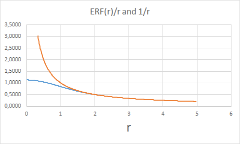
For the description of the location swarm by the field, the Green’s function blurs the location density distribution of the swarm. If the location density distribution has the form of a Gaussian distribution, then the blurred function is the convolution of this location density distribution and the Green’s function.

The Gaussian distribution is

$\rho (r)={\frac {1}{(\sigma {\sqrt {2\pi }})^{3}}}\exp(-{\frac {r^{2}}{2\sigma ^{2}}})$

(41)

The shape of this example is given by:

${\mathfrak {T}}(r)={\frac {1}{4\pi }}{\frac {ERF({\frac {r}{\sigma {\sqrt {2}}}})}{r}}$

(42)

In this function, every trace of the singularity of the Green’s function has disappeared. It is due to the distribution and the huge number of participating hop locations. This shape is just an example.

Such extra potentials add a local contribution to the field that acts as the living space of modules and modular systems.

The shown extra contribution is due to the local elementary module that the swarm represents.

Together, a myriad of such bumps constitutes the living space.

• 
  Potential of a Gaussian distribution

Thus, for a Gaussian location distribution of point-like artifacts the corresponding contribution to field $\psi$ equals an error function divided by its argument. .

Force raising field

From the differential equations, it is not directly clear how fields can raise forces, A second look at these equations might elucidate how fields act forces on discrete objects.

Assume that a uniformly moving coherent swarm corresponds to a shape keeping scalar potential $\varphi (x)$.that resides on a uniformly moving platform. With respect to the background parameter space this scalar potential represents a vector potential ${\vec {\psi }}={\vec {v}}\,\varphi$. Further $\psi _{r}=\varphi$.

At some distance from the center, the scalar potential behaves as

$\varphi \approx {\frac {Q_{1}}{|r|}}$

(43)

${\vec {\nabla }}\varphi \approx {\frac {Q_{1}\,{\vec {r}}}{|r|^{3}}}$

(44)

Now we consider the situation that the total change $\phi =\nabla \,\psi$ of field $\psi$ equals zero

$\phi ={\color {Red}\nabla _{r}\psi _{r}-\langle {\vec {\nabla }},{\vec {\psi }}\rangle +}\nabla _{r}{\vec {\psi }}+{\vec {\nabla }}\psi _{r}{\color {Red}\pm {\vec {\nabla }}\times {\vec {\psi }}}$

(45)

Also, we expect that the red terms equal zero. We also assume that the field is curl-free.

${\vec {\nabla }}\times {\vec {\psi }}=0$

(46)

$\nabla _{r}{\vec {\psi }}=-{\vec {\nabla }}\psi _{r}$

(47)

$\nabla _{r}\,{\vec {\psi }}=(\nabla _{r}\,{\vec {v}})\,\varphi ={\vec {a}}\,\varphi$

(48)

${\vec {\nabla }}\psi _{r}={\vec {\nabla }}\varphi \approx {\frac {Q_{1}\,{\vec {r}}}{|r|^{3}}}$

(49)

${\vec {E}}={\frac {Q_{1}\,{\vec {r}}}{|r|^{3}}}={\vec {a}}\,{\frac {Q_{1}}{|r|}}$

(50)

In those condions the acceleration ${\vec {a}}$ of the swarm produces an extra field ${\vec {E}}$.

For another charge $Q_{2}$ this field ${\vec {E}}$ produces a force ${\vec {F}}={\vec {E}}\ Q_{2}$.

$F({\vec {r}}_{2}-{\vec {r}}_{1})=E({\vec {r}}_{2}-{\vec {r}}_{1})\,Q_{2}\approx {\frac {Q_{1}\,Q_{2}\,({\vec {r}}_{2}-{\vec {r}}_{1})}{|{\vec {r}}_{2}-{\vec {r}}_{1}|^{3}}}$

(51)

Inertia

Equation (51) indicates that acceleration of an embedded object is counteracted by the embedding field.

Lorentz transform

The shock fronts move with speed $c$. In the quaternionic setting, this speed is unity.

$x^{2}+y^{2}+z^{2}=c^{2}t^{2}$

(52)

Swarms of clamp triggers move with lower speed $v$.

For the geometric centers of these swarms still holds:

$x^{2}+y^{2}+z^{2}-c^{2}t^{2}=x'^{2}+y'^{2}+z'^{2}-c^{2}t'^{2}$

(53)

If the locations $\{x,y,z\}$ and $\{x',y',z'\}$ move with uniform relative speed $v$, then

$c\,t'=c\,t\cosh(\omega )-x\sinh(\omega )$

(54)

$\{x,y,x\}$

$x'=x\cosh(\omega )-c\,t\sinh(\omega )$

(55)

$\cosh(\omega )={\frac {\exp(\omega )+\exp(-\omega )}{2}}={\frac {c}{\sqrt {c^{2}-v^{2}}}}$

(56)

$\sinh(\omega )={\frac {\exp(\omega )-\exp(-\omega )}{2}}={\frac {v}{\sqrt {c^{2}-v^{2}}}}$

(57)

$\cosh(\omega )^{2}-\sinh(\omega )^{2}=1$

(58)

This is a hyperbolic transformation that relates two coordinate systems.

This transformation can concern two platforms $P$ and $P'$ on which swarms reside and that move with uniform relative speed $v$.

However, it can also concern the storage location $P$ that contains timestamp $\tau$ and spatial location $\{x,y,z\}$ and platform $P'$ that has coordinate time $t'$ and location $\{x',y',z'\}$.

In this way, the hyperbolic transform relates two individual platforms on which the private swarms of individual elementary particles reside.

It also relates the stored data of an elementary particle and the observed format of these data for the elementary particle that moves with speed $v$ relative to the background parameter space.

The Lorentz transform converts an Euclidean coordinate system consisting of a locations $\{x,y,z\}$ and proper time stamps $\tau$ into the perceived coordinate system that consist of the spacetime coordinates $\{x,y,z,t\}$ in which $t$plays the role of coordinate time. The uniform velocity $v$ causes time dilation $\bigtriangleup t={\frac {\bigtriangleup \tau }{\sqrt {1-{\frac {v^{2}}{c^{2}}}}}}$ and length contraction $\bigtriangleup L=\bigtriangleup L'}{\sqrt {1-{\frac {v^{2}}{c^{2}}}}$. 

Material penetrating field

Basic fields can penetrate homogeneous regions of material. Within these regions, the fields get crumpled. Consequently, the average speed of warps, clamps, and waves diminish or these vibrations just get dampened away.

The basic field that we consider here is a smoothed version ${\widehat {\psi }}$ of the original field $\psi$ that penetrates the material.

${\vec {\varphi }}=\nabla _{r}{\vec {\psi }}+{\vec {\nabla }}{\psi }_{r}\pm {\vec {\nabla }}\times {\vec {\psi }}=\mp {\vec {B}}-{\vec {E}}$

${\vec {\phi }}=\nabla _{r}{\vec {\widehat {\psi }}}+{\vec {\nabla }}{\widehat {\psi }}_{r}\pm {\vec {\nabla }}\times {\vec {\widehat {\psi }}}=\mp {\vec {\mathfrak {B}}}-{\vec {\mathfrak {E}}}$

The first order partial differential equation does not change much. The separate terms in the first order differential equations must be corrected by a material-dependent factor and extra material dependent terms appear.

These extra terms correspond to polarization ${\vec {P}}$ and magnetization ${\vec {M}}$ of the material and the factors concern the permittivity $\epsilon$ and the permeability $\mu$ of the material.

This results in corrections in the ${\vec {\mathfrak {E}}}$ and the ${\vec {\mathfrak {B}}}$ field and the average speed of warps and waves reduces from 1 to $v={\frac {1}{\sqrt {\epsilon \mu }}}$.

${\vec {D}}=\epsilon {\vec {\mathfrak {E}}}+{\vec {P}}$

(59)

${\vec {H}}={\frac {1}{\mu }}{\vec {\mathfrak {B}}}-{\vec {M}}$

(60)

$\rho _{b}=-\langle {\vec {\nabla }},{\vec {P}}\rangle$

(61)

$\rho _{f}=-\langle {\vec {\nabla }},{\vec {D}}\rangle$

(62)

${\vec {J}}_{b}={\vec {\nabla }}\times {\vec {M}}+\nabla _{r}{\vec {P}}$

(63)

${\vec {J}}_{f}={\vec {\nabla }}\times {\vec {H}}-\nabla _{r}{\vec {D}}$

(64)

The subscript $_{b}$ signifies bounded. The subscript $_{f}$ signifies free.

$\rho ={\frac {1}{\epsilon }}\langle {\vec {\nabla }},{\vec {\mathfrak {E}}}\rangle =\rho _{b}+\rho _{f}$

(65)

${\vec {J}}={\frac {1}{\mu }}{\vec {\nabla }}\times {\vec {\mathfrak {B}}}-{\frac {\epsilon }{\mu }}\nabla _{r}{\vec {\mathfrak {E}}}={\vec {J}}_{b}+{\vec {J}}_{f}$

(66)

${\vec {\phi }}={\vec {\mathfrak {E}}}-{\vec {\mathfrak {B}}}={\frac {1}{\epsilon }}({\vec {D}}-{\vec {P}})-\mu ({\vec {H}}+{\vec {M}})$

(67)

The homogeneous second order partial differential equations hold for the smoothed field ${\widehat {\psi }}$.

$\{\nabla _{r}\nabla _{r}\pm v^{2}\langle {\vec {\nabla }},{\vec {\nabla }}\rangle \}{\widehat {\psi }}=0$

(68)

Poynting vector

The Poynting vector represents the directional energy flux density (the rate of energy transfer per unit area) of a basic field.

The quaternionic equivalent of the Poynting vector is defined as:

${\vec {S}}={\vec {E}}\times {\vec {H}}$

(69)

$u$ is the electromagnetic energy density for linear, nondispersive materials, given by

$u={\frac {\langle {\vec {E}},{\vec {B}}\rangle +\langle {\vec {B}},{\vec {H}}\rangle }{2}}$

(70)

${\frac {\partial u}{\partial t}}=-\langle {\vec {\nabla }},{\vec {S}}\rangle -\langle {\vec {J}}_{f},{\vec {E}}\rangle$

(71)