>back to Chapters of Fluid Mechanics for MAP
>back to Chapters of Microfluid Mechanics
Differential Approach: We seek solution at every point
(
x
1
,
x
2
,
x
3
)
{\displaystyle \displaystyle (x_{1},x_{2},x_{3})}
Integral Approach: We focus on a control volume (CV), which is a finite region. It determines gross flow effects such as force or torque on a body or the total energy exchange. For this purpose, balances of incoming and outgoing flux of mass, momentum and energy are made through this finite region. It gives very fast engineering answers, sometimes crude but useful.
Flow over an airfoil: Lagrangian vs Eulerian approach and differential vs integral approach. Lagrangian versus Eulerian Approach: Substantial Derivative [ edit | edit source ] Path of a fluid element Let
α
{\displaystyle \displaystyle \alpha }
α
{\displaystyle \displaystyle \alpha }
(
x
i
)
{\displaystyle \displaystyle (x_{i})}
x
i
{\displaystyle \displaystyle x_{i}}
P
(
x
1
,
x
2
,
x
3
,
t
)
{\displaystyle \displaystyle P(x_{1},x_{2},x_{3},t)}
U
j
(
x
1
,
t
)
,
P
(
x
1
,
t
)
,
ρ
(
x
1
,
t
)
,
T
(
x
1
)
,
τ
j
k
(
x
1
,
t
)
⇒
α
(
x
i
,
t
)
{\displaystyle \displaystyle U_{j}(x_{1},t),P(x_{1},t),\rho (x_{1},t),T(x_{1}),\tau _{jk}(x_{1},t)\Rightarrow \alpha (x_{i},t)}
Lagrangian approach tracks a fluid particle and determines its properties as it moves.
x
i
|
p
(
t
+
Δ
t
)
=
x
i
|
p
(
t
)
+
∫
t
t
+
Δ
t
U
i
|
p
(
t
′
)
d
t
′
{\displaystyle \displaystyle x_{i}|_{p}(t+\Delta t)=x_{i}|_{p}(t)+\int _{t}^{t+\Delta t}U_{i}|_{p}(t')dt'}
Oceanographic measurements made with floating sensors delivering location, pressure and temperature data, is one example of this approach. X-ray opaque dyes, which are used to trace blood flow in arteries, is another example.
Let
α
p
{\displaystyle \displaystyle \alpha _{p}}
α
p
{\displaystyle \displaystyle \alpha _{p}}
For this variable:
α
p
(
x
p
→
,
t
)
{\displaystyle \displaystyle \alpha _{p}({\vec {x_{p}}},t)}
x
p
→
=
x
p
→
(
t
)
→
α
p
(
x
p
→
,
t
)
=
α
p
(
t
)
{\displaystyle \displaystyle {\vec {x_{p}}}={\vec {x_{p}}}(t)\rightarrow \alpha _{p}({\vec {x_{p}}},t)=\alpha _{p}(t)}
α
{\displaystyle \displaystyle \alpha }
In a fluid flow, due to excessive number of fluid particles, Lagrangian approach is not widely used.
Thus, for a particle P finding itself at point
x
i
{\displaystyle \displaystyle x_{i}}
α
p
(
t
)
=
α
[
(
x
i
)
p
,
t
]
{\displaystyle \displaystyle \alpha _{p}(t)=\alpha \left[(x_{i})_{p},t\right]}
Along the path of the particle:
α
p
(
t
+
Δ
t
)
=
α
[
(
x
i
+
Δ
x
i
)
p
,
t
+
Δ
t
]
{\displaystyle \displaystyle \alpha _{p}(t+\Delta t)=\alpha \left[(x_{i}+\Delta x_{i})_{p},t+\Delta t\right]}
d
α
p
=
α
[
(
(
x
i
+
Δ
x
i
)
p
,
t
+
Δ
t
)
−
α
(
(
x
i
)
p
,
t
)
]
{\displaystyle \displaystyle d\alpha _{p}=\alpha \left[((x_{i}+\Delta x_{i})_{p},t+\Delta t)-\alpha ((x_{i})_{p},t)\right]}
d
α
p
=
∂
α
∂
t
d
t
+
∂
α
∂
x
i
d
x
i
p
{\displaystyle \displaystyle d\alpha _{p}={\frac {\partial \alpha }{\partial t}}dt+{\frac {\partial \alpha }{\partial x_{i}}}dx_{ip}}
d
α
p
d
t
=
∂
α
∂
t
+
(
∂
α
∂
x
i
)
(
d
x
i
d
t
)
p
=
∂
α
∂
t
⏟
L
o
c
a
l
c
h
a
n
g
e
i
n
t
i
m
e
+
∂
α
∂
x
i
U
i
⏟
C
h
a
n
g
e
i
n
s
p
a
c
e
{\displaystyle \displaystyle {\frac {d\alpha _{p}}{dt}}={\frac {\partial \alpha }{\partial t}}+\left({\frac {\partial \alpha }{\partial x_{i}}}\right)\left({\frac {dx_{i}}{dt}}\right)_{p}=\underbrace {\frac {\partial \alpha }{\partial t}} _{Local\ change\ in\ time}+\underbrace {{\frac {\partial \alpha }{\partial x_{i}}}U_{i}} _{Change\ in\ space}}
d
α
p
d
t
=
D
α
D
t
=
(
∂
∂
t
+
U
i
∂
∂
x
i
)
α
{\displaystyle \displaystyle {\frac {d\alpha _{p}}{dt}}={\frac {D\alpha }{Dt}}=\left({\frac {\partial }{\partial t}}+U_{i}{\frac {\partial }{\partial x_{i}}}\right)\alpha }
In mechanics, system is a collection of matter of fixed identity (always the same atoms or fluid particles) which may move, flow and interact with its surroundings.
Hence, the mass is constant for a system, although it may continually change size and shape. This approach is very useful in statics and dynamics, in which the system can be isolated from its surrounding and its interaction with the surrounding can be analysed by using a free-body diagram.
In fluid dynamics, it is very hard to identify and follow a specific quantity of the fluid. Imagine a river and you have to follow a specific mass of water along the river.
Mostly, we are rather interested in determining forces on surfaces, for example on the surfaces of airplanes and cars. Hence, instead of system approach, we identify a specific volume in space (associated with our geometry of interest) and analyse the flow within, through or around this volume. This specific volume is called "Control Volume". This control volume can be fixed, moving or even deforming.
The control volume is a specific geometric entity independent of the flowing fluid. The matter within a control volume may change with time, and the mass may not remain constant.
Example of different types of control volume. A)Fixed CV: Flow through a pipe. B)Moving CV: Flow through a jet engine of a flying aircraft C)Deforming CV: Flow from a deflating balloon The mass of a system do not change:
d
M
d
t
s
y
s
t
e
m
|
=
0
{\displaystyle \displaystyle \displaystyle {\frac {dM}{dt}}_{system}{\bigg |}=0}
M
=
∫
m
a
s
s
(
s
y
s
t
e
m
)
d
m
=
∫
V
(
s
y
s
t
e
m
)
ρ
d
V
{\displaystyle \displaystyle \displaystyle M=\int _{mass(system)}{dm}=\int _{V(system)}{\rho dV}}
For a system moving relative to a inertial reference frame, the sum of all external forces acting on the system is equal to the time rate of change of linear momentum (
P
→
{\displaystyle \displaystyle {\vec {P}}}
F
i
=
d
P
i
d
t
|
s
y
s
t
e
m
{\displaystyle \displaystyle F_{i}={\frac {dP_{i}}{dt}}{\bigg |}_{system}}
P
i
(
s
y
s
t
e
m
)
=
∫
m
a
s
s
(
s
y
s
t
e
m
)
U
i
d
m
=
∫
V
(
s
y
s
t
e
m
)
U
i
ρ
d
V
{\displaystyle \displaystyle \displaystyle P_{i(system)}=\int _{mass(system)}{U_{i}dm}=\int _{V(system)}{U_{i}\rho dV}}
d
Q
⏟
h
e
a
t
a
d
d
e
d
o
n
s
y
s
t
e
m
+
d
W
⏟
w
o
r
k
d
o
n
e
o
n
s
y
s
t
e
m
=
d
E
{\displaystyle \displaystyle \underbrace {dQ} _{heat\ added\ on\ system}+\underbrace {dW} _{work\ done\ on\ system}=dE}
Q
˙
+
W
˙
=
d
E
d
t
|
s
y
s
t
e
m
{\displaystyle \displaystyle {\dot {Q}}+{\dot {W}}={\frac {dE}{dt}}{\bigg |}_{system}}
E
s
y
s
t
e
m
=
∫
m
a
s
s
(
s
y
s
t
e
m
)
e
d
m
=
∫
V
(
s
y
s
t
e
m
)
e
ρ
d
V
{\displaystyle \displaystyle \displaystyle E_{system}=\int _{mass(system)}{edm}=\int _{V(system)}{e\rho dV}}
e
=
u
⏟
I
n
t
e
n
r
a
l
e
n
e
r
g
y
+
U
i
U
i
2
⏟
K
i
n
e
t
i
c
e
n
e
r
g
y
+
g
z
⏟
P
o
t
e
n
t
i
a
l
e
n
e
r
g
y
{\displaystyle \displaystyle \displaystyle e=\underbrace {u} _{Intenral\ energy}+\underbrace {\frac {U_{i}U_{i}}{2}} _{Kinetic\ energy}+\underbrace {gz} _{Potential\ energy}}
moment of momentum (angular momentum) and second law of thermodynamics , but they are not the subject of this course and will not be treated here.
Note that all basic laws are written for a system, i.e defined mass with fixed identity. We should rephrase these laws for a control volume.
Relation of a system derivative to the control volume derivative [ edit | edit source ]
Consider a fire extinguisher
d
M
d
t
|
s
y
s
t
e
m
=
0
{\displaystyle \displaystyle {\frac {dM}{dt}}{\bigg |}_{system}=0}
whereas
d
M
d
t
|
c
v
<
0
{\displaystyle \displaystyle {\frac {dM}{dt}}{\bigg |}_{cv}<0}
We would like to relate
d
B
d
t
|
s
y
s
t
e
m
{\displaystyle \displaystyle {\frac {dB}{dt}}{\bigg |}_{system}}
d
B
d
t
|
c
v
{\displaystyle \displaystyle {\frac {dB}{dt}}{\bigg |}_{cv}}
The variables appear in the physical laws (balance laws) of a system are:
Mass (
M
{\displaystyle \displaystyle M}
Momentum (
P
i
{\displaystyle \displaystyle P_{i}}
Energy (
E
{\displaystyle \displaystyle E}
Moment of momentum (
H
i
{\displaystyle \displaystyle H_{i}}
Entropy (
S
{\displaystyle \displaystyle S}
They are called extensive properties. Let
B
{\displaystyle \displaystyle B}
b
{\displaystyle \displaystyle b}
B
s
y
s
t
e
m
=
∫
m
a
s
s
(
s
y
s
t
e
m
)
b
d
m
=
∫
V
(
s
y
s
t
e
m
)
b
ρ
d
V
{\displaystyle \displaystyle B_{system}=\int _{mass(system)}{b\ dm}=\int _{V(system)}{b\rho dV}}
B
=
M
,
b
=
1
{\displaystyle \displaystyle B=M,\ b=1}
B
=
P
→
,
b
=
u
→
{\displaystyle \displaystyle B={\vec {P}},\ b={\vec {u}}}
B
=
E
,
b
=
e
{\displaystyle \displaystyle B=E,\ b=e}
Control Volume versus System
Flow through a nozzle used to derive the 1-D Reynolds transport theorem Consider a flow through a nozzle.
If
B
{\displaystyle \displaystyle B}
B
s
y
s
(
t
)
=
B
c
v
(
t
)
{\displaystyle \displaystyle B_{sys}(t)=B_{cv}(t)}
B
s
y
s
(
t
+
Δ
t
)
=
B
c
v
(
t
+
Δ
t
)
−
B
I
(
t
+
Δ
t
)
+
B
I
I
(
t
+
Δ
t
)
{\displaystyle \displaystyle \displaystyle B_{sys}(t+\Delta t)=B_{cv}(t+\Delta t)-B_{I}(t+\Delta t)+B_{II}(t+\Delta t)}
Δ
B
s
y
s
Δ
t
=
B
s
y
s
(
t
+
Δ
t
)
−
B
s
y
s
(
t
)
Δ
t
=
B
c
v
(
t
+
Δ
t
)
−
B
c
v
(
t
)
Δ
t
−
B
I
(
t
+
Δ
t
)
Δ
t
+
B
I
I
(
t
+
Δ
t
)
Δ
t
{\displaystyle \displaystyle {\frac {\Delta B_{sys}}{\Delta t}}={\frac {B_{sys}(t+\Delta t)-B_{sys}(t)}{\Delta t}}={\frac {B_{cv}(t+\Delta t)-B_{cv}(t)}{\Delta t}}\ -\ {\frac {B_{I}(t+\Delta t)}{\Delta t}}\ +\ {\frac {B_{II}(t+\Delta t)}{\Delta t}}}
Δ
t
→
0
{\displaystyle \displaystyle \Delta t\rightarrow 0}
lim
Δ
t
→
0
B
c
v
(
t
+
Δ
t
)
−
B
c
v
(
t
)
Δ
t
=
∂
B
c
v
∂
t
{\displaystyle \displaystyle \lim _{\Delta t\rightarrow 0}{\frac {B_{cv}(t+\Delta t)-B_{cv}(t)}{\Delta t}}={\frac {\partial B_{cv}}{\partial t}}}
B
I
I
(
t
+
Δ
t
)
{\displaystyle \displaystyle B_{II}(t+\Delta t)}
Δ
t
→
0
{\displaystyle \displaystyle \Delta t\rightarrow 0}
B
I
I
(
t
+
Δ
t
)
=
ρ
2
b
2
Δ
V
2
{\displaystyle \displaystyle B_{II}(t+\Delta t)=\rho _{2}b_{2}\Delta V_{2}}
B
I
I
(
t
+
Δ
t
)
=
ρ
2
b
2
A
2
l
2
=
ρ
2
b
2
A
2
U
2
Δ
t
{\displaystyle \displaystyle \displaystyle B_{II}(t+\Delta t)=\rho _{2}b_{2}A_{2}l_{2}=\rho _{2}b_{2}A_{2}U_{2}\Delta t}
B
o
u
t
=
ρ
2
b
2
A
2
U
2
Δ
t
{\displaystyle \displaystyle \displaystyle B_{out}=\rho _{2}b_{2}A_{2}U_{2}\Delta t}
B
I
(
t
+
Δ
t
)
=
ρ
1
b
1
Δ
V
1
=
ρ
1
b
1
A
1
U
1
Δ
t
=
B
i
n
{\displaystyle \displaystyle \displaystyle B_{I}(t+\Delta t)=\rho _{1}b_{1}\Delta V_{1}=\rho _{1}b_{1}A_{1}U_{1}\Delta t=B_{in}}
Δ
t
→
0
{\displaystyle \displaystyle \Delta t\rightarrow 0}
Δ
B
s
y
s
Δ
t
→
d
B
s
y
s
d
t
{\displaystyle \displaystyle {\frac {\Delta B_{sys}}{\Delta t}}\rightarrow {\frac {dB_{sys}}{dt}}}
B
i
n
Δ
t
=
B
˙
i
n
{\displaystyle \displaystyle {\frac {B_{in}}{\Delta t}}={\dot {B}}_{in}}
B
o
u
t
Δ
t
=
B
˙
o
u
t
{\displaystyle \displaystyle {\frac {B_{out}}{\Delta t}}={\dot {B}}_{out}}
so that,
d
B
s
y
s
d
t
=
∂
B
c
v
∂
t
+
B
˙
o
u
t
−
B
˙
i
n
{\displaystyle \displaystyle {\frac {dB_{sys}}{dt}}={\frac {\partial B_{cv}}{\partial t}}+{\dot {B}}_{out}-{\dot {B}}_{in}}
The three terms on the RHS of RTT are:
1. The rate of change of B within CV indicates the local unsteady effect.
2. The flux of B passing out of the CS.
3. The flux of B passing into the CS.
There can be more than one inlet and outlet.
Hence, for a quite complex, unsteady, three dimensional situation, we need a more general form of RTT. Consider an arbitrary 3-D CV and the outward unit normal vector
(
n
→
)
{\displaystyle ({\vec {n}})}
B
{\displaystyle B}
B
˙
o
u
t
=
∫
C
S
o
u
t
d
B
o
u
t
=
∫
C
S
o
u
t
ρ
b
U
→
⋅
n
→
d
A
{\displaystyle \displaystyle {\dot {B}}_{out}=\int _{CSout}{dB_{out}}=\int _{CSout}{\rho b{\vec {U}}\cdot {\vec {n}}dA}}
B
˙
i
n
=
∫
C
S
i
n
d
B
i
n
=
−
∫
C
S
i
n
ρ
b
U
→
⋅
n
→
d
A
{\displaystyle \displaystyle {\dot {B}}_{in}=\int _{CSin}{dB_{in}}=-\int _{CSin}{\rho b{\vec {U}}\cdot {\vec {n}}dA}}
B
˙
i
n
{\displaystyle \displaystyle {\dot {B}}_{in}}
B
˙
o
u
t
{\displaystyle \displaystyle {\dot {B}}_{out}}
B
˙
i
n
{\displaystyle \displaystyle {\dot {B}}_{in}}
U
→
⋅
n
→
{\displaystyle \displaystyle {\vec {U}}\cdot {\vec {n}}}
d
B
s
y
s
d
t
=
∂
B
c
v
∂
t
+
∫
C
S
o
u
t
ρ
b
U
→
⋅
n
→
d
A
+
∫
C
S
i
n
ρ
b
U
→
⋅
n
→
d
A
{\displaystyle \displaystyle {\frac {dB_{sys}}{dt}}={\frac {\partial B_{cv}}{\partial t}}+\int _{CSout}{\rho b{\vec {U}}\cdot {\vec {n}}dA}+\int _{CSin}{\rho b{\vec {U}}\cdot {\vec {n}}dA}}
d
B
s
y
s
d
t
=
∂
∂
t
∫
c
v
ρ
b
d
V
+
∫
c
s
ρ
b
U
→
⋅
n
→
d
A
{\displaystyle \displaystyle {\frac {dB_{sys}}{dt}}={\frac {\partial }{\partial t}}\int _{cv}{\rho bdV}+\int _{cs}{\rho b{\vec {U}}\cdot {\vec {n}}dA}}
Since
ρ
u
→
⋅
n
→
d
A
=
d
m
{\displaystyle \displaystyle \rho {\vec {u}}\cdot {\vec {n}}dA=dm}
d
B
s
y
s
d
t
=
∂
B
c
v
∂
t
+
∫
C
S
b
d
m
⏟
n
e
t
f
l
u
x
o
f
B
a
c
r
o
s
s
C
S
{\displaystyle \displaystyle {\frac {dB_{sys}}{dt}}={\frac {\partial B_{cv}}{\partial t}}+\underbrace {\int _{CS}{bdm}} _{net\ flux\ of\ B\ across\ CS}}
It is possible that CV can move with constant velocity or arbitrary acceleration.
This form of RTT is valid if the CV has no acceleration with respect to a fixed (inertial) reference frame. RTT is then valid for a moving CV with constant velocity when:
1. All velocities are measured relative to the CV.
2. All time derivative measure relative to the CV.
U
→
s
{\displaystyle \displaystyle {\vec {U}}_{s}}
U
→
r
=
U
→
−
U
→
s
{\displaystyle \displaystyle {\vec {U}}_{r}={\vec {U}}-{\vec {U}}_{s}}
d
B
s
y
s
d
t
=
d
d
t
(
∫
c
v
b
ρ
d
V
)
+
∫
c
s
b
ρ
U
r
→
⋅
n
→
d
A
{\displaystyle \displaystyle {\frac {dB_{sys}}{dt}}={\frac {d}{dt}}\left(\int _{cv}{b\rho dV}\right)+\int _{cs}{b\rho {\vec {U_{r}}}\cdot {\vec {n}}dA}}
CV with multiple inlets and outlets CV with arbitrary shape used to derive Reynolds transport theorem Sign of the inflow and outflow fluxes to the CV Relation between the absolute velocity vector with the velocity of the moving reference frame and the velocity w.r.t. to the moving reference frame
B
=
M
,
b
=
1
{\displaystyle \displaystyle B=M,b=1}
d
M
s
y
s
d
t
=
∂
∂
t
∫
c
v
b
ρ
d
V
+
∫
c
s
b
ρ
U
→
⋅
n
→
d
A
=
0
{\displaystyle \displaystyle {\frac {dM_{sys}}{dt}}={\frac {\partial }{\partial t}}\int _{cv}{b\rho dV}+\int _{cs}{b\rho {\vec {U}}\cdot {\vec {n}}dA}=0}
∂
∂
t
∫
c
v
ρ
d
V
⏟
r
a
t
e
o
f
c
h
a
n
g
e
o
f
m
a
s
s
i
n
C
V
+
∫
c
s
ρ
U
→
⋅
n
→
d
A
⏟
n
e
t
r
a
t
e
o
f
m
a
s
s
f
l
u
x
t
h
r
o
u
g
h
t
h
e
C
S
=
0
{\displaystyle \displaystyle \underbrace {{\frac {\partial }{\partial t}}\int _{cv}{\rho dV}} _{rate\ of\ change\ of\ mass\ in\ CV}+\underbrace {\int _{cs}{\rho {\vec {U}}\cdot {\vec {n}}dA}} _{net\ rate\ of\ mass\ flux\ through\ the\ CS}=0}
ρ
{\displaystyle \displaystyle \rho }
0
=
ρ
∂
∂
t
∫
c
v
d
V
+
ρ
∫
c
s
U
→
⋅
n
→
d
A
{\displaystyle \displaystyle 0=\rho {\frac {\partial }{\partial t}}\int _{cv}{dV}+\rho \int _{cs}{{\vec {U}}\cdot {\vec {n}}dA}}
V
{\displaystyle \displaystyle V}
0
=
ρ
∫
c
s
U
→
⋅
n
→
d
A
→
∫
c
s
U
→
⋅
n
→
d
A
⏟
v
o
l
u
m
e
f
l
o
w
r
a
t
e
=
0
{\displaystyle \displaystyle 0=\rho \int _{cs}{{\vec {U}}\cdot {\vec {n}}dA}\rightarrow \underbrace {\int _{cs}{{\vec {U}}\cdot {\vec {n}}dA}} _{volume\ flow\ rate}=0}
Note that we did not assume a steady flow. This equation is valid for both steady and unsteady flows.
If the flow is steady,
0
=
∫
c
s
ρ
U
→
⋅
n
→
d
A
→
Net mass flow rate is equal to zero
{\displaystyle \displaystyle 0=\int _{cs}{\rho {\vec {U}}\cdot {\vec {n}}dA}\rightarrow {\text{Net mass flow rate is equal to zero}}}
there is no-mass accumulation or deficit in the control volume.
B
=
P
→
{\displaystyle \displaystyle B={\vec {P}}}
b
=
U
→
{\displaystyle \displaystyle b={\vec {U}}}
d
P
→
d
t
s
y
s
t
e
m
=
∂
∂
t
∫
c
v
U
→
ρ
d
V
+
∫
c
s
U
→
ρ
U
→
⋅
n
→
d
A
⏟
m
o
m
e
n
t
u
m
f
l
u
x
{\displaystyle \displaystyle {\frac {d{\vec {P}}}{dt}}_{system}={\frac {\partial }{\partial t}}\int _{cv}{{\vec {U}}\rho dV}+\underbrace {\int _{cs}{{\vec {U}}\rho {\vec {U}}\cdot {\vec {n}}dA}} _{momentum\ flux}}
d
P
→
d
t
s
y
s
t
e
m
=
F
→
o
n
s
y
s
t
e
m
{\displaystyle \displaystyle {\frac {d{\vec {P}}}{dt}}_{system}={\vec {F}}_{on\ system}}
Force on the system is the sum of surface forces and body forces.
F
→
o
n
s
y
s
t
e
m
=
F
S
→
+
F
B
→
{\displaystyle \displaystyle {\vec {F}}_{on\ system}={\vec {F_{S}}}+{\vec {F_{B}}}}
The surface forces are mainly due to pressure, which is normal to the surface, and viscous stresses, which can be both normal or tangential to the surfaces.
F
→
p
r
e
s
s
u
r
e
=
−
∫
A
P
n
→
d
A
{\displaystyle \displaystyle {\vec {F}}_{pressure}=-\int _{A}{P{\vec {n}}dA}}
F
→
v
.
s
t
r
e
s
s
e
s
=
∫
A
τ
d
A
{\displaystyle \displaystyle {\vec {F}}_{v.stresses}=\int _{A}{\tau dA}}
The body forces can be due to gravity or magnetic field.
at the initial moment
t
{\displaystyle \displaystyle t}
F
→
o
n
s
y
s
t
e
m
=
F
→
o
n
C
V
{\displaystyle \displaystyle {\vec {F}}_{on\ system}={\vec {F}}_{on\ CV}}
F
S
i
+
F
B
i
=
∂
∂
t
∫
c
v
U
i
ρ
d
V
+
∫
c
s
U
i
ρ
U
j
n
j
d
A
{\displaystyle \displaystyle F_{Si}+F_{Bi}={\frac {\partial }{\partial t}}\int _{cv}{U_{i}\rho dV}+\int _{cs}{U_{i}\rho U_{j}n_{j}dA}}
B
=
E
,
b
=
e
{\displaystyle \displaystyle B=E,b=e}
d
E
d
t
s
y
s
t
e
m
=
∂
∂
t
∫
c
v
e
ρ
d
V
+
∫
c
s
e
ρ
U
→
⋅
n
→
d
A
{\displaystyle \displaystyle {\frac {dE}{dt}}_{system}={\frac {\partial }{\partial t}}\int _{cv}{e\rho dV}+\int _{cs}{e\rho {\vec {U}}\cdot {\vec {n}}dA}}
t
{\displaystyle \displaystyle t}
d
E
d
t
s
y
s
t
e
m
=
[
Q
˙
+
W
˙
]
s
y
s
t
e
m
=
[
Q
˙
+
W
˙
]
c
v
{\displaystyle \displaystyle {\frac {dE}{dt}}_{system}=[{\dot {Q}}+{\dot {W}}]_{system}=[{\dot {Q}}+{\dot {W}}]_{cv}}
thus, the integral form of energy equation is:
[
Q
˙
+
W
˙
]
c
v
=
∂
∂
t
∫
c
v
e
ρ
d
V
+
∫
c
s
e
ρ
U
→
⋅
n
→
d
A
{\displaystyle \displaystyle [{\dot {Q}}+{\dot {W}}]_{cv}={\frac {\partial }{\partial t}}\int _{cv}{e\rho dV}+\int _{cs}{e\rho {\vec {U}}\cdot {\vec {n}}dA}}
Consider the mass balance in a stream tube by using the integral form of the conservatin of mass equation.
Let
A
1
{\displaystyle \displaystyle A_{1}}
A
2
{\displaystyle \displaystyle A_{2}}
U
→
{\displaystyle \displaystyle {\vec {U}}}
A
1
{\displaystyle \displaystyle A_{1}}
A
2
{\displaystyle \displaystyle A_{2}}
∂
∂
t
∫
c
v
ρ
d
V
+
∫
c
s
ρ
U
→
⋅
n
→
d
A
=
0
{\displaystyle \displaystyle {\frac {\partial }{\partial t}}\int _{cv}{\rho dV}+\int _{cs}{\rho {\vec {U}}\cdot {\vec {n}}dA}=0}
∫
C
S
I
ρ
U
→
⋅
n
→
d
A
+
∫
C
S
I
I
I
ρ
U
→
⋅
n
→
d
A
+
∫
C
S
I
I
ρ
U
→
⋅
n
→
d
A
=
0
{\displaystyle \displaystyle \int _{CS_{I}}{\rho {\vec {U}}\cdot {\vec {n}}dA}+\int _{CS_{III}}{\rho {\vec {U}}\cdot {\vec {n}}}dA+\int _{CS_{II}}{\rho {\vec {U}}\cdot {\vec {n}}dA}=0}
C
S
I
I
I
{\displaystyle \displaystyle CS_{III}}
−
ρ
U
1
A
1
+
0
+
ρ
U
2
A
2
=
0
{\displaystyle \displaystyle \displaystyle -\rho U_{1}A_{1}+0+\rho U_{2}A_{2}=0}
ρ
U
1
A
1
=
ρ
U
2
A
2
→
U
2
=
U
1
A
1
A
2
{\displaystyle \displaystyle \rho U_{1}A_{1}=\rho U_{2}A_{2}\rightarrow U_{2}={\frac {U_{1}A_{1}}{A_{2}}}}
m
˙
1
=
m
˙
2
{\displaystyle \displaystyle {\dot {m}}_{1}={\dot {m}}_{2}}
Mass balance for stream tube inside a laminar flow
Consider the steady flow of water through the device. The inlet and outlet areas are
A
1
{\displaystyle \displaystyle A_{1}}
A
2
{\displaystyle \displaystyle A_{2}}
A
3
{\displaystyle \displaystyle A_{3}}
A
4
{\displaystyle \displaystyle A_{4}}
The following parameters are known:
Mass flow out at 3 (
m
˙
3
{\displaystyle \displaystyle {\dot {m}}_{3}}
Volume flow rate in through 4 (
Q
4
{\displaystyle \displaystyle {Q}_{4}}
Velocity at 1 along
x
1
{\displaystyle \displaystyle x_{1}}
U
→
11
{\displaystyle \displaystyle {\vec {U}}_{11}}
U
→
1
i
=
(
U
11
,
0
,
0
)
{\displaystyle \displaystyle {\vec {U}}_{1i}=(U_{11},0,0)}
U
11
>
0
{\displaystyle \displaystyle U_{11}>0}
Find the flow velocity at section 2?Assume that the properties are uniform across the sections.
∂
∂
t
∫
c
v
ρ
d
V
+
∫
c
s
ρ
U
→
⋅
n
→
d
A
=
0
{\displaystyle \displaystyle {\frac {\partial }{\partial t}}\int _{cv}{\rho dV}+\int _{cs}{\rho {\vec {U}}\cdot {\vec {n}}dA}=0}
∫
A
1
ρ
U
→
1
⋅
n
→
1
d
A
=
−
ρ
|
U
11
|
A
1
{\displaystyle \displaystyle \int _{A_{1}}{\rho {\vec {U}}_{1}\cdot {\vec {n}}_{1}dA}=-\rho \left|U_{11}\right|A_{1}}
∫
A
3
ρ
U
→
3
⋅
n
→
3
d
A
=
ρ
|
U
3
|
A
3
=
m
˙
3
{\displaystyle \displaystyle \int _{A_{3}}{\rho {\vec {U}}_{3}}\cdot {\vec {n}}_{3}dA=\rho \left|U_{3}\right|A_{3}={\dot {m}}_{3}}
∫
A
4
ρ
U
→
4
⋅
n
→
4
d
A
=
−
ρ
|
U
4
|
A
4
=
−
ρ
Q
4
{\displaystyle \displaystyle \int _{A_{4}}{\rho {\vec {U}}_{4}\cdot {\vec {n}}_{4}dA}=-\rho \left|U_{4}\right|A_{4}=-\rho Q_{4}}
∫
A
1
ρ
U
→
1
⋅
n
→
1
d
A
+
∫
A
2
ρ
U
→
2
⋅
n
→
2
d
A
+
∫
A
3
ρ
U
→
3
⋅
n
→
3
d
A
+
∫
A
4
ρ
U
→
4
⋅
n
→
4
d
A
=
0
{\displaystyle \displaystyle \int _{A_{1}}{\rho {\vec {U}}_{1}\cdot {\vec {n}}_{1}dA}+\int _{A_{2}}{\rho {\vec {U}}_{2}\cdot {\vec {n}}_{2}}dA+\int _{A_{3}}{\rho {\vec {U}}_{3}\cdot {\vec {n}}_{3}dA}+\int _{A_{4}}{\rho {\vec {U}}_{4}\cdot {\vec {n}}_{4}dA}=0}
mass balance for a connector device Hence, the velocity at section 2 can be calculated by
∫
A
2
ρ
U
→
2
⋅
n
→
2
d
A
=
−
[
−
ρ
|
U
1
|
A
1
+
m
˙
3
−
ρ
Q
4
]
{\displaystyle \displaystyle \int _{A_{2}}{\rho {\vec {U}}_{2}\cdot {\vec {n}}_{2}dA}=-\left[-\rho \left|U_{1}\right|A_{1}+{\dot {m}}_{3}-\rho Q_{4}\right]}
n
→
2
=
(
0
,
−
1
)
→
U
21
=
0
{\displaystyle \displaystyle {\vec {n}}_{2}=(0,-1)\rightarrow U_{21}=0}
−
ρ
U
22
A
2
=
ρ
|
U
1
|
A
1
−
m
→
3
+
ρ
Q
4
{\displaystyle \displaystyle -\rho U_{22}A_{2}=\rho \left|U_{1}\right|A_{1}-{\vec {m}}_{3}+\rho Q_{4}}
U
2
{\displaystyle \displaystyle U_{2}}
U
2
{\displaystyle \displaystyle U_{2}}
F
i
=
F
S
i
+
F
B
i
=
∂
∂
t
∫
c
v
U
i
ρ
d
V
+
∫
c
s
U
i
ρ
U
j
n
j
d
A
{\displaystyle \displaystyle F_{i}=F_{Si}+F_{Bi}={\frac {\partial }{\partial t}}\int _{cv}{U_{i}\rho dV}+\int _{cs}{U_{i}\rho U_{j}n_{j}dA}}
F
i
=
∫
C
S
I
U
1
i
ρ
U
1
j
n
j
d
A
+
∫
C
S
I
I
U
2
i
ρ
U
2
j
n
j
d
A
{\displaystyle \displaystyle \displaystyle F_{i}=\int _{CS_{I}}{U_{1i}\rho U_{1j}n_{j}dA}+\int _{CS_{II}}{U_{2i}\rho U_{2j}n_{j}dA}}
F
i
=
−
U
1
i
|
U
→
1
|
A
1
ρ
⏟
m
˙
1
+
U
2
i
|
U
→
2
|
A
2
ρ
2
⏟
m
˙
2
{\displaystyle \displaystyle F_{i}=-U_{1i}\underbrace {\left|{\vec {U}}_{1}\right|A_{1}\rho } _{{\dot {m}}_{1}}\ +\ U_{2i}\underbrace {\left|{\vec {U}}_{2}\right|A_{2}\rho _{2}} _{{\dot {m}}_{2}}}
m
˙
1
=
m
˙
2
=
m
˙
{\displaystyle \displaystyle {\dot {m}}_{1}={\dot {m}}_{2}={\dot {m}}}
F
i
=
m
˙
(
U
2
i
−
U
1
i
)
{\displaystyle \displaystyle F_{i}={\dot {m}}(U_{2i}-U_{1i})}
Force in a streamtube
Experimental Setup for nozzle test Water from a stationary nozzle strikes to a plate. Assume that the flow is normal to the plate and in the jet velocity is uniform. Determine the force on the plate in
x
1
{\displaystyle \displaystyle x_{1}}
0
=
∫
c
s
ρ
U
i
n
i
d
A
(
m
a
s
s
)
{\displaystyle \displaystyle 0=\int _{cs}{\rho U_{i}n_{i}dA}\ (mass)}
F
i
=
F
S
i
+
F
B
i
=
∫
c
s
U
i
ρ
U
j
n
j
d
A
(
m
o
m
e
n
t
u
m
)
{\displaystyle \displaystyle F_{i}=F_{Si}+F_{Bi}=\int _{cs}{U_{i}\rho U_{j}n_{j}dA}\ (momentum)}
x
1
{\displaystyle \displaystyle x_{1}}
F
1
=
F
S
1
=
∫
c
s
U
1
ρ
U
j
n
j
d
A
{\displaystyle \displaystyle \displaystyle F_{1}=F_{S1}=\int _{cs}{U_{1}\rho U_{j}n_{j}dA}}
F
S
1
=
p
a
A
−
p
a
A
+
R
1
{\displaystyle \displaystyle \displaystyle F_{S1}=p_{a}A-p_{a}A+R_{1}}
R
1
=
∫
c
s
U
1
ρ
U
j
n
j
d
A
=
∫
C
S
1
U
1
1
ρ
U
j
1
n
j
d
A
+
∫
C
S
2
U
1
2
ρ
U
j
2
n
j
d
A
⏟
0
+
∫
C
S
3
U
1
3
ρ
U
j
3
n
j
d
A
⏟
0
{\displaystyle \displaystyle R_{1}=\int _{cs}{U_{1}\rho U_{j}n_{j}dA}=\int _{CS1}{U_{1}^{1}\rho U_{j}^{1}n_{j}dA}+\underbrace {\int _{CS2}{U_{1}^{2}\rho U_{j}^{2}n_{j}dA}} _{0}+\underbrace {\int _{CS3}{U_{1}^{3}\rho U_{j}^{3}n_{j}dA}} _{0}}
Control volume I and II and Free body diagram of the plate
U
1
=
0
{\displaystyle \displaystyle U_{1}=0}
R
1
=
−
U
1
ρ
U
1
A
J
e
t
{\displaystyle \displaystyle R_{1}=-U_{1}\rho U_{1}A_{Jet}}
K
1
=
−
R
1
=
U
1
ρ
U
1
A
J
e
t
{\displaystyle \displaystyle K_{1}=-R_{1}=U_{1}\rho U_{1}A_{Jet}}
C
V
2
{\displaystyle \displaystyle CV_{2}}
F
S
1
=
p
a
A
+
R
1
=
−
U
1
2
A
j
e
t
ρ
{\displaystyle \displaystyle F_{S1}=p_{a}A+R_{1}=-U_{1}^{2}A_{jet}\rho }
R
1
=
−
p
a
A
−
U
1
2
A
J
e
t
ρ
{\displaystyle \displaystyle R_{1}=-p_{a}A-U_{1}^{2}A_{Jet}\rho }
Hence, the force exerted on the plate by the CV is
K
1
=
−
R
1
{\displaystyle \displaystyle K_{1}=-R_{1}}
F
n
e
t
=
−
R
1
−
p
a
A
{\displaystyle \displaystyle \displaystyle F_{net}=-R_{1}-p_{a}A}
F
n
e
t
=
p
a
A
+
U
1
2
A
ρ
−
p
a
A
{\displaystyle \displaystyle F_{net}=p_{a}A+U_{1}^{2}A\rho -p_{a}A}
F
n
e
t
=
U
1
2
A
ρ
{\displaystyle \displaystyle F_{net}=U_{1}^{2}A\rho }
Velocity distribution of fluid over a plate Consider the plate exposed to uniform velocity. The flow is steady and incompressible. A boundary layer builds up on the plate. Determine the Drag force on the plate. Note that
U
1
{\displaystyle \displaystyle U_{1}}
U
1
(
L
,
x
2
)
=
U
(
2
x
2
δ
−
(
x
2
δ
)
2
)
{\displaystyle \displaystyle U_{1}(L,x_{2})=U\left(2{\frac {x_{2}}{\delta }}-\left({\frac {x_{2}}{\delta }}\right)^{2}\right)}
ρ
∫
c
s
U
i
n
i
d
A
=
0
{\displaystyle \displaystyle \displaystyle \rho \int _{cs}{U_{i}n_{i}dA}=0}
ρ
∫
0
h
−
U
0
w
d
x
2
+
ρ
∫
0
δ
U
w
d
x
2
=
0
{\displaystyle \displaystyle \rho \int _{0}^{h}{-U_{0}\ w\ dx_{2}}+\rho \int _{0}^{\delta }{U\ w\ dx_{2}}=0}
U
0
h
=
∫
0
δ
U
d
x
2
{\displaystyle \displaystyle U_{0}h=\int _{0}^{\delta }{Udx_{2}}}
F
i
=
∂
∂
t
∫
U
i
ρ
d
V
⏟
=
0
s
t
e
a
d
y
s
t
a
t
e
+
∫
c
s
U
i
ρ
U
j
n
j
d
A
{\displaystyle \displaystyle F_{i}=\underbrace {{\frac {\partial }{\partial t}}\int {U_{i}\rho dV}} _{=0\ steady\ state}+\int _{cs}{U_{i}\rho U_{j}n_{j}dA}}
F
1
=
−
D
=
∫
0
h
U
1
ρ
U
j
n
j
d
A
+
∫
C
S
2
U
1
ρ
U
j
n
j
d
A
⏟
=
0
s
t
r
e
a
m
l
i
n
e
+
∫
0
δ
U
1
ρ
U
j
n
j
d
A
+
∫
U
1
ρ
U
j
n
j
d
A
⏟
=
0
w
a
l
l
{\displaystyle \displaystyle F_{1}=-D=\int _{0}^{h}{U_{1}\rho U_{j}n_{j}dA}+\underbrace {\int _{CS2}{U_{1}\rho U_{j}n_{j}dA}} _{=0\ streamline}+\int _{0}^{\delta }{U_{1}\rho U_{j}n_{j}dA}+\underbrace {\int {U_{1}\rho U_{j}n_{j}dA}} _{=0\ wall}}
−
D
=
−
U
0
ρ
U
0
h
w
+
∫
U
1
ρ
U
1
w
d
x
2
{\displaystyle \displaystyle -D=-U_{0}\rho U_{0}\ h\ w+\int {U_{1}\rho U_{1}\ w\ dx_{2}}}
D
=
U
0
2
ρ
h
w
−
ρ
w
∫
0
δ
U
1
2
d
x
2
=
ρ
U
0
∫
0
δ
U
1
d
x
2
−
ρ
w
∫
0
δ
U
0
U
1
d
x
2
{\displaystyle \displaystyle D=U_{0}^{2}\rho \ h\ w-\rho \ w\int _{0}^{\delta }{U_{1}^{2}dx_{2}}=\rho U_{0}\int _{0}^{\delta }{U_{1}dx_{2}}-\rho \ w\int _{0}^{\delta }{U_{0}U_{1}dx_{2}}}
D
=
ρ
w
∫
0
δ
U
1
(
U
0
−
U
1
)
d
x
2
|
x
1
=
L
{\displaystyle \displaystyle D=\rho w\int _{0}^{\delta }{U_{1}(U_{0}-U_{1})dx_{2}}|_{x_{1}=L}}
U
1
{\displaystyle \displaystyle U_{1}}
x
2
δ
=
η
{\displaystyle \displaystyle {\frac {x_{2}}{\delta }}=\eta }
D
=
ρ
w
U
0
2
δ
∫
0
1
(
2
η
−
η
2
)
(
1
−
2
η
+
η
2
)
d
η
=
2
15
ρ
U
0
2
w
δ
{\displaystyle \displaystyle D=\rho \ w\ U_{0}^{2}\delta \int _{0}^{1}{(2\eta -\eta ^{2})(1-2\eta +\eta ^{2})d\eta }={\frac {2}{15}}\rho U_{0}^{2}w\ \delta }
Consider the jet and the vane. Determine the force to be applied such that vane moves with a constant speed
U
→
v
{\displaystyle \displaystyle {\vec {U}}_{v}}
x
1
{\displaystyle \displaystyle x_{1}}
Note that for an inertial CV (static or moving with constant speed) RTT is valid, but velocities should be written with respect to the moving CV.
F
i
=
F
S
i
+
F
B
i
⏟
=
0
=
∂
∂
t
∫
c
v
U
i
ρ
d
V
⏟
=
0
(steady)
+
∫
c
s
U
i
ρ
U
j
n
j
d
A
{\displaystyle \displaystyle F_{i}=F_{S_{i}}+\underbrace {F_{B_{i}}} _{=0}=\underbrace {{\frac {\partial }{\partial t}}\int _{cv}{U_{i}\rho dV}} _{=0{\textrm {(steady)}}}+\int _{cs}{U_{i}\rho U_{j}n_{j}dA}}
F
S
i
=
R
1
+
p
a
A
−
p
a
A
{\displaystyle \displaystyle F_{S_{i}}=R_{1}+p_{a}A-p_{a}A}
R
1
=
∫
c
s
U
1
ρ
U
j
n
j
d
A
{\displaystyle \displaystyle \displaystyle R_{1}=\int _{cs}{U_{1}\rho U_{j}n_{j}dA}}
R
1
=
−
U
1
1
ρ
|
U
→
1
|
A
1
+
U
1
2
ρ
|
U
→
2
|
A
2
{\displaystyle \displaystyle \displaystyle R_{1}=-U_{1}^{1}\rho \left|{\vec {U}}^{1}\right|A_{1}+U_{1}^{2}\rho \left|{\vec {U}}^{2}\right|A_{2}}
=
(
U
1
2
−
U
1
)
m
˙
(
(
|
U
→
j
e
t
|
)
−
|
U
→
v
|
(
cos
θ
−
1
)
)
{\displaystyle \displaystyle =(U_{1}^{2}-U_{1}){\dot {m}}((\left|{\overrightarrow {U}}_{jet}\right|)-\left|{\overrightarrow {U}}_{v}\right|(\cos \theta \ -1))}
from continuity,
0
=
∫
c
s
ρ
U
⋅
n
d
A
=
−
|
U
→
1
|
ρ
A
1
+
|
U
→
2
|
ρ
A
2
{\displaystyle \displaystyle 0=\int _{cs}{\rho U\cdot ndA}=-\left|{\vec {U}}^{1}\right|\rho A_{1}+\left|{\vec {U}}^{2}\right|\rho A_{2}}
ρ
|
U
→
1
|
A
1
=
ρ
|
U
→
2
|
A
2
→
m
˙
{\displaystyle \displaystyle \rho \left|{\vec {U}}^{1}\right|A_{1}=\rho \left|{\vec {U}}^{2}\right|A_{2}\rightarrow {\dot {m}}}
R
1
=
(
U
1
2
−
U
1
)
ρ
|
U
1
|
A
1
{\displaystyle \displaystyle R_{1}=(U_{1}^{2}-U_{1})\rho \left|U^{1}\right|A_{1}}
|
U
1
|
=
|
U
→
j
e
t
−
U
→
v
|
{\displaystyle \displaystyle \left|U^{1}\right|=\left|{\vec {U}}_{jet}-{\vec {U}}_{v}\right|}
U
1
1
=
|
U
→
j
e
t
|
−
|
U
→
v
|
{\displaystyle \displaystyle U_{1}^{1}=\left|{\vec {U}}_{jet}\right|-\left|{\vec {U}}_{v}\right|}
U
1
2
=
(
|
U
→
j
e
t
|
−
|
U
→
v
|
)
c
o
s
θ
{\displaystyle \displaystyle U_{1}^{2}=\left(\left|{\vec {U}}_{jet}\right|-\left|{\vec {U}}_{v}\right|\right)cos\theta }
for
A
1
=
A
2
{\displaystyle A_{1}=A_{2}}
R
1
=
ρ
(
|
U
→
j
e
t
|
−
|
U
→
v
|
)
2
(
c
o
s
θ
−
1
)
A
1
{\displaystyle \displaystyle R_{1}=\rho \left(\left|{\vec {U}}_{jet}\right|-\left|{\vec {U}}_{v}\right|\right)^{2}\left(cos\theta -1\right)A_{1}}
=
(
U
1
2
−
U
i
)
m
˙
(
(
|
U
→
j
e
t
|
)
−
(
|
U
→
v
|
)
)
{\displaystyle \displaystyle =(U_{1}^{2}-U_{i}){\dot {m}}((\left|{\overrightarrow {U}}_{jet}\right|)-(\left|{\overrightarrow {U}}_{v}\right|))}
R
2
=
∫
c
s
U
2
ρ
U
j
n
j
d
A
{\displaystyle \displaystyle \displaystyle R_{2}=\int _{cs}{U_{2}\rho U_{j}n_{j}dA}}
R
2
=
∫
A
1
U
2
1
ρ
U
j
2
n
j
2
d
A
+
∫
A
2
U
2
2
ρ
U
j
2
n
j
2
d
A
{\displaystyle \displaystyle R_{2}=\int _{A_{1}}{U_{2}^{1}\rho U_{j}^{2}n_{j}^{2}dA}+\int _{A_{2}}{U_{2}^{2}\rho U_{j}^{2}n_{j}^{2}dA}}
U
2
1
=
0
{\displaystyle \displaystyle U_{2}^{1}=0}
U
2
2
=
|
U
→
2
|
s
i
n
θ
{\displaystyle \displaystyle U_{2}^{2}=\left|{\vec {U}}^{2}\right|sin\theta }
R
2
=
∫
A
2
U
2
2
ρ
U
j
2
n
j
2
d
A
{\displaystyle \displaystyle R_{2}=\int _{A_{2}}{U_{2}^{2}\rho U_{j}^{2}n_{j}^{2}dA}}
R
2
=
U
2
2
ρ
|
U
→
2
|
A
2
{\displaystyle \displaystyle R_{2}=U_{2}^{2}\rho \left|{\vec {U}}_{2}\right|A_{2}}
R
2
=
|
U
→
2
|
2
ρ
s
i
n
θ
A
2
{\displaystyle \displaystyle R_{2}=\left|{\vec {U}}^{2}\right|^{2}\rho \ sin\theta A_{2}}
|
U
→
1
|
=
|
U
→
2
|
=
|
U
→
j
e
t
−
U
→
v
|
{\displaystyle \displaystyle \left|{\vec {U}}^{1}\right|=\left|{\vec {U}}^{2}\right|=\left|{\vec {U}}_{jet}-{\vec {U}}_{v}\right|}
U
→
=
U
→
j
e
t
−
U
→
v
{\displaystyle \displaystyle {\vec {U}}={\vec {U}}_{jet}-{\vec {U}}_{v}}
For an inertial CV the following transport equation for momentum holds:
F
→
=
∂
∂
t
∫
c
v
U
→
ρ
d
V
+
∫
c
s
U
→
ρ
U
→
⋅
n
→
d
A
{\displaystyle \displaystyle {\vec {F}}={\frac {\partial }{\partial t}}\int _{cv}{{\vec {U}}\rho \ dV}+\int _{cs}{{\vec {U}}\rho {\vec {U}}\cdot {\vec {n}}dA}}
Denote an inertial reference frame with
X
1
,
X
2
,
X
3
{\displaystyle \displaystyle X_{1},X_{2},X_{3}}
x
1
,
x
2
,
x
3
{\displaystyle \displaystyle x_{1},x_{2},x_{3}}
x
1
,
x
2
,
x
3
{\displaystyle \displaystyle x_{1},x_{2},x_{3}}
non-inertial frame of reference . Let the system to move with a velocity and an acceleration
U
→
r
f
{\displaystyle \displaystyle {\vec {U}}_{rf}}
a
→
r
f
{\displaystyle \displaystyle {\vec {a}}_{rf}}
U
→
X
=
U
→
x
+
U
→
r
f
{\displaystyle \displaystyle {\overrightarrow {U}}_{X}={\overrightarrow {U}}_{x}+{\overrightarrow {U}}_{rf}}
d
U
→
X
d
t
=
d
U
→
x
d
t
+
d
U
→
r
f
d
t
⇒
d
U
→
X
d
t
≠
d
U
→
x
d
t
{\displaystyle \displaystyle {\frac {d{\overrightarrow {U}}_{X}}{dt}}={\frac {d{\overrightarrow {U}}_{x}}{dt}}+{\frac {d{\overrightarrow {U}}_{rf}}{dt}}\Rightarrow {\frac {d{\overrightarrow {U}}_{X}}{dt}}\neq {\frac {d{\overrightarrow {U}}_{x}}{dt}}}
or,
a
→
X
=
a
→
x
+
a
→
r
f
⇒
d
P
→
X
d
t
≠
d
P
→
x
d
t
{\displaystyle \displaystyle {\vec {a}}_{X}={\vec {a}}_{x}+{\vec {a}}_{rf}\Rightarrow {\frac {d{\overrightarrow {P}}_{X}}{dt}}\neq {\frac {d{\overrightarrow {P}}_{x}}{dt}}}
These above relationship implies that the velocity and the acceleration is not same when considered from inertial and moving reference frame.
The Newton's second law states that:
F
→
|
s
y
s
t
e
m
=
d
P
→
X
d
t
|
s
y
s
t
e
m
{\displaystyle \displaystyle \left.{\vec {F}}\right|_{system}=\left.{\frac {d{\vec {P}}_{X}}{dt}}\right|_{system}}
U
→
x
=
U
→
X
−
U
→
r
f
{\displaystyle \displaystyle {\vec {U}}_{x}={\vec {U}}_{X}-{\vec {U}}_{rf}}
U
→
x
{\displaystyle \displaystyle {\vec {U}}_{x}}
U
→
X
{\displaystyle \displaystyle {\vec {U}}_{X}}
d
U
→
x
d
t
=
d
U
→
X
d
t
−
d
U
→
r
f
d
t
(
1
)
{\displaystyle \displaystyle {\frac {d{\vec {U}}_{x}}{dt}}={\frac {d{\vec {U}}_{X}}{dt}}-{\frac {d{\vec {U}}_{rf}}{dt}}(1)}
a
→
x
=
a
→
X
−
a
→
r
f
{\displaystyle \displaystyle {\vec {a}}_{x}={\vec {a}}_{X}-{\vec {a}}_{rf}}
U
→
r
f
{\displaystyle \displaystyle {\vec {U}}_{rf}}
a
→
r
f
{\displaystyle \displaystyle {\vec {a}}_{rf}}
d
U
→
C
V
d
t
=
d
U
→
r
f
d
t
{\displaystyle \displaystyle {\frac {d{\vec {U}}_{CV}}{dt}}={\frac {d{\vec {U}}_{rf}}{dt}}}
d
U
c
v
d
t
≠
0
{\displaystyle \displaystyle {\frac {dU_{cv}}{dt}}\neq 0}
P
→
X
{\displaystyle \displaystyle {\vec {P}}_{X}}
P
→
x
{\displaystyle \displaystyle {\vec {P}}_{x}}
To develop momentum equation for an accelerating CV, it is necessary to relate
P
→
X
{\displaystyle \displaystyle {\vec {P}}_{X}}
P
→
x
{\displaystyle \displaystyle {\vec {P}}_{x}}
Previously we have seen that in a non-inertial reference frame having rectilinear acceleration, i.e. (translational acceleration).
a
→
X
=
a
→
x
+
a
→
r
f
{\displaystyle \displaystyle {\vec {a}}_{X}={\vec {a}}_{x}+{\vec {a}}_{rf}}
and also
F
→
=
∫
m
a
s
s
(
s
y
s
t
e
m
)
a
→
X
d
m
{\displaystyle \displaystyle {\vec {F}}=\int _{mass\ (system)}{{\vec {a}}_{X}dm}}
=
∫
m
a
s
s
(
s
y
s
t
e
m
)
(
a
→
x
+
a
→
r
f
)
d
m
{\displaystyle \displaystyle =\int _{mass\ (system)}{({\vec {a}}_{x}+{\vec {a}}_{rf})dm}}
F
→
−
∫
m
a
s
s
(
s
y
s
t
e
m
)
a
→
r
f
d
m
=
∫
m
a
s
s
(
s
y
s
t
e
m
)
a
→
x
d
m
{\displaystyle \displaystyle {\vec {F}}-\int _{mass\ (system)}{{\vec {a}}_{rf}dm}=\int _{mass\ (system)}{{\vec {a}}_{x}dm}}
F
→
−
∫
m
a
s
s
(
s
y
s
t
e
m
)
a
→
r
f
d
m
=
∫
m
a
s
s
(
s
y
s
t
e
m
)
d
U
→
x
d
t
d
m
=
d
d
t
∫
m
a
s
s
(
s
y
s
t
e
m
)
U
→
x
d
m
{\displaystyle \displaystyle {\vec {F}}-\int _{mass\ (system)}{{\vec {a}}_{rf}dm}=\int _{mass\ (system)}{{\frac {d{\vec {U}}_{x}}{dt}}dm}={\frac {d}{dt}}\int _{mass\ (system)}{{\vec {U}}_{x}dm}}
F
→
−
∫
V
(
s
y
s
t
e
m
)
a
→
r
f
ρ
d
V
=
d
P
→
x
d
t
|
s
y
s
t
e
m
{\displaystyle \displaystyle {\vec {F}}-\int _{V\ (system)}{{\vec {a}}_{rf}\rho \ dV}={\frac {d{\vec {P}}_{x}}{dt}}|_{system}}
d
P
→
x
d
t
|
s
y
s
t
e
m
=
∂
∂
t
∫
c
v
U
→
x
ρ
d
V
+
∫
c
s
U
→
x
ρ
U
→
x
⋅
n
→
d
A
{\displaystyle \displaystyle {\frac {d{\vec {P}}_{x}}{dt}}|_{system}={\frac {\partial }{\partial t}}\int _{cv}{{\vec {U}}_{x}\rho \ dV}+\int _{cs}{{\vec {U}}_{x}\rho {\vec {U}}_{x}\cdot {\vec {n}}dA}}
t
0
{\displaystyle \displaystyle t_{0}}
F
→
o
n
s
y
s
t
e
m
−
∫
V
s
y
s
t
e
m
a
→
r
f
ρ
d
V
=
F
→
o
n
c
v
−
∫
c
v
a
→
r
f
ρ
d
V
{\displaystyle \displaystyle {\vec {F}}_{on\ system}-\int _{V\ system}{{\vec {a}}_{rf}\rho dV}={\vec {F}}_{on\ cv}-\int _{cv}{{\vec {a}}_{rf}\rho dV}}
F
→
o
n
c
v
−
∫
c
v
a
→
r
f
ρ
d
V
=
∂
∂
t
∫
c
v
U
→
x
ρ
d
V
+
∫
c
s
U
→
x
ρ
U
→
x
⋅
n
→
d
A
{\displaystyle \displaystyle {\vec {F}}_{on\ cv}-\int _{cv}{{\vec {a}}_{rf}\rho dV}={\frac {\partial }{\partial t}}\int _{cv}{{\vec {U}}_{x}\rho \ dV}+\int _{cs}{{\vec {U}}_{x}\rho {\vec {U}}_{x}\cdot {\vec {n}}dA}}
A small rocket, with an inertial mass of
M
0
{\displaystyle \displaystyle M_{0}}
m
˙
{\displaystyle \displaystyle {\dot {m}}}
U
e
{\displaystyle \displaystyle U_{e}}
Neglecting drag on the rocket, find the relation for the velocity of the rocket U(t).
F
2
⏟
A
−
∫
c
v
a
→
r
f
2
ρ
d
V
⏟
B
=
∂
∂
t
∫
c
v
U
→
2
ρ
d
V
⏟
C
+
∫
c
s
U
2
ρ
U
→
x
⋅
n
→
d
V
⏟
D
{\displaystyle \displaystyle \underbrace {F_{2}} _{A}-\underbrace {\int _{cv}{{\vec {a}}_{rf2}\rho dV}} _{B}=\underbrace {{\frac {\partial }{\partial t}}\int _{cv}{{\vec {U}}_{2}\rho dV}} _{C}+\underbrace {\int _{cs}{U_{2}\rho {\vec {U}}_{x}\cdot {\vec {n}}dV}} _{D}}
F
2
=
−
g
∫
c
v
ρ
d
V
=
−
g
M
c
v
{\displaystyle \displaystyle F_{2}=-g\int _{cv}{\rho dV}=-g\ M_{cv}}
M
c
v
=
M
0
−
m
˙
t
{\displaystyle \displaystyle M_{cv}=M_{0}-{\dot {m}}t}
F
2
=
−
g
(
M
0
−
m
˙
t
)
{\displaystyle \displaystyle F_{2}=-g(M_{0}-{\dot {m}}t)}
a
→
r
f
{\displaystyle \displaystyle {\vec {a}}_{rf}}
−
∫
c
v
a
r
f
2
ρ
d
V
=
−
a
r
f
2
∫
c
v
ρ
d
V
{\displaystyle \displaystyle \displaystyle -\int _{cv}{a_{rf2}\rho dV}=-a_{rf2}\int _{cv}{\rho dV}}
−
∫
c
v
a
r
f
2
ρ
d
V
=
−
a
r
f
2
(
M
0
−
m
˙
t
)
{\displaystyle \displaystyle -\int _{cv}{a_{rf2}\rho dV}=-a_{rf2}(M_{0}-{\dot {m}}t)}
is the time rate of change at
x
2
{\displaystyle \displaystyle x_{2}}
∂
∂
t
∫
c
v
U
2
ρ
d
V
=
∂
∂
t
∫
c
v
I
U
2
ρ
d
V
+
∂
∂
t
∫
c
v
I
I
U
2
ρ
d
V
{\displaystyle \displaystyle {\frac {\partial }{\partial t}}\int _{cv}{U_{2}\rho dV}={\frac {\partial }{\partial t}}\int _{cvI}{U_{2}\rho dV}+{\frac {\partial }{\partial t}}\int _{cvII}{U_{2}\rho dV}}
U
2
=
−
U
e
{\displaystyle \displaystyle U_{2}=-U_{e}}
∂
∂
t
[
∫
C
V
I
U
2
ρ
d
V
⏟
U
2
=
0
→=
0
+
∫
C
V
I
I
U
2
ρ
d
V
]
=
∂
∂
t
∫
C
V
I
I
U
2
ρ
d
V
≈
0
{\displaystyle \displaystyle {\frac {\partial }{\partial t}}\left[\underbrace {\int _{CVI}{U_{2}\rho dV}} _{U_{2}=0\rightarrow =0}+\int _{CVII}{U_{2}\rho dV}\right]={\frac {\partial }{\partial t}}\int _{CVII}{U_{2}\rho dV}\approx 0}
D:
∫
c
s
U
2
ρ
U
→
x
⋅
n
→
d
A
=
U
2
∫
c
s
ρ
U
→
x
⋅
n
→
d
A
=
U
2
m
˙
=
−
U
e
m
˙
{\displaystyle \displaystyle \int _{cs}{U_{2}\rho {\vec {U}}_{x}\cdot {\vec {n}}dA}=U_{2}\int _{cs}{\rho {\vec {U}}_{x}\cdot {\vec {n}}dA}=U_{2}{\dot {m}}=-U_{e}{\dot {m}}}
−
g
(
M
0
−
m
˙
t
)
−
a
r
f
2
(
M
0
−
m
˙
t
)
=
−
U
e
m
˙
{\displaystyle \displaystyle -g(M_{0}-{\dot {m}}t)-a_{rf2}(M_{0}-{\dot {m}}t)=-U_{e}{\dot {m}}}
a
r
f
2
=
U
e
m
˙
M
0
−
m
˙
t
−
g
{\displaystyle \displaystyle a_{rf2}={\frac {U_{e}{\dot {m}}}{M_{0}-{\dot {m}}t}}-\ g}
d
V
c
v
d
t
=
a
r
f
2
=
U
e
m
˙
M
0
−
m
˙
t
−
g
{\displaystyle \displaystyle {\frac {dV_{cv}}{dt}}=a_{rf2}={\frac {U_{e}{\dot {m}}}{M_{0}-{\dot {m}}t}}-\ g}
V
c
v
(
t
)
=
∫
0
t
U
e
m
˙
M
0
−
m
˙
t
d
t
−
∫
0
t
g
d
t
{\displaystyle \displaystyle V_{cv}(t)=\int _{0}^{t}{\frac {U_{e}{\dot {m}}}{M_{0}-{\dot {m}}t}}dt-\int _{0}^{t}gdt}
V
c
v
(
t
)
=
−
U
e
l
n
(
1
−
m
˙
t
M
0
)
−
g
t
{\displaystyle \displaystyle V_{cv}(t)=-U_{e}ln\left(1-{\frac {{\dot {m}}t}{M_{0}}}\right)-gt}
l
n
{\displaystyle \displaystyle ln}
Control Volume I and II
[
Q
˙
+
W
˙
]
o
n
s
y
s
t
e
m
=
[
Q
˙
+
W
˙
]
o
n
c
v
=
∂
∂
t
∫
e
ρ
d
V
+
∫
c
s
e
ρ
U
→
⋅
n
→
d
A
{\displaystyle \displaystyle \left[{\dot {Q}}+{\dot {W}}\right]_{on\ system}=\left[{\dot {Q}}+{\dot {W}}\right]_{on\ cv}={\frac {\partial }{\partial t}}\int {e\rho \ dV}+\int _{cs}{e\rho {\vec {U}}\cdot {\vec {n}}dA}}
e
=
U
+
|
U
→
|
2
2
+
g
z
{\displaystyle \displaystyle e=U+{\frac {\left|{\vec {U}}\right|^{2}}{2}}+g\ z}
W
˙
o
n
c
v
=
W
˙
b
o
d
y
+
W
˙
s
u
r
f
a
c
e
{\displaystyle \displaystyle {\dot {W}}_{on\ cv}={\dot {W}}_{body}+{\dot {W}}_{surface}}
z
=
x
2
{\displaystyle \displaystyle z=x_{2}}
W
˙
b
o
d
y
=
W
˙
s
h
a
f
t
+
W
˙
e
l
e
c
+
W
˙
o
t
h
e
r
{\displaystyle \displaystyle {\dot {W}}_{body}={\dot {W}}_{shaft}+{\dot {W}}_{elec}+{\dot {W}}_{other}}
W
˙
s
u
r
f
a
c
e
=
W
˙
n
o
r
m
a
l
+
W
˙
s
h
e
a
r
{\displaystyle \displaystyle {\dot {W}}_{surface}={\dot {W}}_{normal}+{\dot {W}}_{shear}}
τ
→
s
{\displaystyle \displaystyle {\vec {\tau }}_{s}}
τ
→
n
{\displaystyle \displaystyle {\vec {\tau }}_{n}}
τ
→
n
=
−
p
n
→
d
A
{\displaystyle \displaystyle {\vec {\tau }}_{n}=-p{\vec {n}}dA}
W
˙
=
F
→
⋅
U
→
{\displaystyle \displaystyle {\dot {W}}={\vec {F}}\cdot {\vec {U}}}
d
W
˙
=
d
F
→
⋅
U
→
{\displaystyle \displaystyle d{\dot {W}}=d{\vec {F}}\cdot {\vec {U}}}
d
W
˙
n
o
r
m
a
l
=
τ
→
n
d
A
⋅
U
→
→
W
˙
n
o
r
m
a
l
=
∫
c
s
τ
→
n
⋅
U
→
d
A
=
−
∫
c
s
p
n
→
⋅
U
→
d
A
{\displaystyle \displaystyle d{\dot {W}}_{normal}={\vec {\tau }}_{n}dA\cdot {\vec {U}}\rightarrow {\dot {W}}_{normal}=\int _{cs}{{\vec {\tau }}_{n}\cdot {\vec {U}}dA}=-\int _{cs}{p{\vec {n}}\cdot {\vec {U}}dA}}
d
W
˙
s
h
e
a
r
=
τ
→
d
A
⋅
U
→
→
W
˙
s
h
e
a
r
=
∫
c
s
τ
→
⋅
U
→
d
A
{\displaystyle \displaystyle d{\dot {W}}_{shear}={\vec {\tau }}dA\cdot {\vec {U}}\rightarrow {\dot {W}}_{shear}=\int _{cs}{{\vec {\tau }}\cdot {\vec {U}}dA}}
Q
˙
+
W
˙
s
h
a
f
t
+
W
˙
s
h
e
a
r
+
W
˙
o
t
h
e
r
=
∂
∂
t
∫
e
ρ
d
V
+
∫
c
s
(
u
+
p
ρ
⏟
h
:
e
n
t
h
a
l
p
y
+
|
U
→
2
|
2
+
g
x
2
)
ρ
U
→
⋅
n
→
d
A
{\displaystyle \displaystyle {\dot {Q}}\ +\ {\dot {W}}_{shaft}\ +\ {\dot {W}}_{shear}\ +\ {\dot {W}}_{other}={\frac {\partial }{\partial t}}\int {e\rho dV}+\int _{cs}{\left(\underbrace {u+{\frac {p}{\rho }}} _{h:\ enthalpy}+{\frac {\left|{\vec {U}}^{2}\right|}{2}}+gx_{2}\right)\rho {\vec {U}}\cdot {\vec {n}}dA}}
Shear and Normal stress component on the surface element dA /
P
i
n
p
u
t
{\displaystyle \displaystyle P_{input}}
V
˙
{\displaystyle \displaystyle {\dot {V}}}
Find a relation for the rate of heat transfer in terms of the power, temperature, pressure, etc.
Q
˙
+
W
˙
s
h
a
f
t
+
W
˙
s
h
e
a
r
⏟
=
0
=
τ
⋅
U
→
+
W
˙
o
t
h
e
r
⏟
=
0
=
∂
∂
t
∫
e
ρ
d
V
⏟
=
0
s
t
e
a
d
y
s
t
a
t
e
+
∫
c
s
(
u
+
p
ρ
+
U
2
2
+
g
x
2
)
ρ
U
→
⋅
n
→
d
A
{\displaystyle \displaystyle {\dot {Q}}\ +\ {\dot {W}}_{shaft}+\underbrace {{\dot {W}}_{shear}} _{=\ 0\ =\tau \cdot {\vec {U}}}+\underbrace {{\dot {W}}_{other}} _{=\ 0}=\underbrace {{\frac {\partial }{\partial t}}\int {}e\rho dV} _{=\ 0\ steady\ state}+\int _{cs}{\left(u+{\frac {p}{\rho }}+{\frac {U^{2}}{2}}+gx_{2}\right)\rho {\vec {U}}\cdot {\vec {n}}dA}}
0
=
∂
∂
t
∫
c
v
ρ
d
V
⏟
=
0
s
t
e
a
d
y
s
t
a
t
e
+
∫
c
s
ρ
U
→
⋅
n
→
d
A
→
|
ρ
1
U
1
A
1
|
=
|
ρ
2
U
2
A
2
|
=
m
˙
{\displaystyle \displaystyle 0=\underbrace {{\frac {\partial }{\partial t}}\int _{cv}{\rho dV}} _{=\ 0\ steady\ state}+\int _{cs}{\rho {\vec {U}}\cdot {\vec {n}}dA}\rightarrow \left|\rho _{1}U_{1}A_{1}\right|=\left|\rho _{2}U_{2}A_{2}\right|={\dot {m}}}
Q
˙
=
−
W
˙
s
h
a
f
t
+
∫
c
s
(
u
+
p
ρ
+
U
2
2
+
g
z
)
ρ
U
→
⋅
n
→
d
A
{\displaystyle \displaystyle {\dot {Q}}=-{\dot {W}}_{shaft}+\int _{cs}{\left(u+{\frac {p}{\rho }}+{\frac {U^{2}}{2}}+gz\right)\rho {\vec {U}}\cdot {\vec {n}}dA}}
enthalpy
h
=
u
+
p
ρ
{\displaystyle \displaystyle h=u+{\frac {p}{\rho }}}
Q
˙
=
−
W
˙
s
h
a
f
t
−
(
h
1
+
U
1
2
2
⏟
=
0
+
g
z
1
)
|
ρ
1
U
1
A
1
|
+
(
h
2
+
U
2
2
2
+
g
z
2
)
|
ρ
2
A
2
U
2
|
{\displaystyle \displaystyle {\dot {Q}}=-{\dot {W}}_{shaft}-\left(h_{1}+\underbrace {\frac {U_{1}^{2}}{2}} _{=\ 0}+gz_{1}\right)\left|\rho _{1}U_{1}A_{1}\right|+\left(h_{2}+{\frac {U_{2}^{2}}{2}}+gz_{2}\right)\left|\rho _{2}A_{2}U_{2}\right|}
Q
˙
=
−
W
˙
s
h
a
f
t
+
m
˙
[
h
2
+
U
2
2
2
−
h
1
+
g
(
z
2
−
z
1
)
⏟
=
0
]
{\displaystyle \displaystyle {\dot {Q}}=-{\dot {W}}_{shaft}+{\dot {m}}\left[h_{2}+{\frac {U_{2}^{2}}{2}}-h_{1}+\underbrace {g(z_{2}-z_{1})} _{=\ 0}\right]}
c
p
{\displaystyle \displaystyle c_{p}}
h
2
−
h
1
=
c
p
(
T
2
−
T
1
)
{\displaystyle \displaystyle \displaystyle h_{2}-h_{1}=c_{p}(T_{2}-T_{1})}
Q
˙
=
−
W
˙
s
h
a
f
t
+
m
˙
[
c
p
(
T
2
−
T
1
)
+
U
2
2
2
]
{\displaystyle \displaystyle {\dot {Q}}=-{\dot {W}}_{shaft}+{\dot {m}}\left[c_{p}(T_{2}-T_{1})+{\frac {U_{2}^{2}}{2}}\right]}
Energy balance for a compressor
For a CV with one inlet 1, one outlet 2 and steady uniform flow through it.
Q
˙
+
W
˙
s
h
a
f
t
+
W
˙
s
h
e
a
r
⏟
K
=
∫
c
s
(
u
+
p
ρ
+
|
U
→
2
|
2
+
g
z
)
ρ
U
→
⋅
n
→
d
A
{\displaystyle \displaystyle \underbrace {{\dot {Q}}+{\dot {W}}_{shaft}+{\dot {W}}_{shear}} _{K}=\int _{cs}{\left(u+{\frac {p}{\rho }}+{\frac {\left|{\vec {U}}^{2}\right|}{2}}+gz\right)\rho {\vec {U}}\cdot {\vec {n}}dA}}
K
=
(
u
1
+
p
1
ρ
1
+
|
U
→
1
2
|
2
+
g
z
1
)
∫
1
ρ
1
U
→
1
⋅
n
→
d
A
⏟
−
m
˙
+
(
u
2
+
p
2
ρ
2
+
|
U
→
2
2
|
2
+
g
z
2
)
∫
2
ρ
2
U
→
2
⋅
n
→
d
A
⏟
m
˙
{\displaystyle \displaystyle K=\left(u_{1}+{\frac {p_{1}}{\rho _{1}}}+{\frac {\left|{\vec {U}}_{1}^{2}\right|}{2}}+gz_{1}\right)\underbrace {\int _{1}{\rho _{1}{\vec {U}}_{1}}\cdot {\vec {n}}dA} _{-{\dot {m}}}+\left(u_{2}+{\frac {p_{2}}{\rho _{2}}}+{\frac {\left|{\vec {U}}_{2}^{2}\right|}{2}}+gz_{2}\right)\underbrace {\int _{2}{\rho _{2}{\vec {U}}_{2}}\cdot {\vec {n}}dA} _{\dot {m}}}
K
=
m
˙
[
(
u
2
−
u
1
)
+
(
p
2
ρ
2
−
p
1
ρ
1
)
+
(
U
→
2
2
2
−
U
→
1
2
2
)
+
g
(
z
2
−
z
1
)
]
{\displaystyle \displaystyle K={\dot {m}}\left[(u_{2}-u_{1})+\left({\frac {p_{2}}{\rho _{2}}}-{\frac {p_{1}}{\rho _{1}}}\right)+\left({\frac {{\vec {U}}_{2}^{2}}{2}}-{\frac {{\vec {U}}_{1}^{2}}{2}}\right)+g(z_{2}-z_{1})\right]}
p
1
ρ
1
+
|
U
→
1
2
|
2
+
g
z
1
=
p
2
ρ
2
+
|
U
→
2
2
|
2
+
g
z
2
+
(
u
2
−
u
1
)
−
Q
˙
m
˙
−
W
˙
s
h
a
f
t
m
˙
−
W
˙
s
h
e
a
r
m
˙
{\displaystyle \displaystyle {\frac {p_{1}}{\rho _{1}}}+{\frac {\left|{\vec {U}}_{1}^{2}\right|}{2}}+gz_{1}={\frac {p_{2}}{\rho _{2}}}+{\frac {\left|{\vec {U}}_{2}^{2}\right|}{2}}+gz_{2}+(u_{2}-u_{1})-{\frac {\dot {Q}}{\dot {m}}}-{\frac {{\dot {W}}_{shaft}}{\dot {m}}}-{\frac {{\dot {W}}_{shear}}{\dot {m}}}}
W
˙
s
h
a
f
t
=
0
{\displaystyle \displaystyle {\dot {W}}_{shaft}=0}
W
˙
s
h
e
a
r
=
0
{\displaystyle \displaystyle {\dot {W}}_{shear}=0}
p
1
ρ
+
|
U
→
1
2
|
2
+
g
z
1
⏟
m
e
c
h
a
n
i
c
a
l
e
v
e
r
g
y
p
e
r
u
n
i
t
m
a
s
s
a
t
f
l
o
w
c
r
o
s
s
s
e
c
t
i
o
n
=
p
2
ρ
+
|
U
→
2
2
|
2
+
g
z
2
+
(
u
2
−
u
1
)
−
Q
˙
m
˙
{\displaystyle \displaystyle \underbrace {{\frac {p_{1}}{\rho }}+{\frac {\left|{\vec {U}}_{1}^{2}\right|}{2}}+gz_{1}} _{mechanical\ evergy\ per\ unit\ mass\ at\ flow\ cross\ section}={\frac {p_{2}}{\rho }}+{\frac {\left|{\vec {U}}_{2}^{2}\right|}{2}}+gz_{2}+(u_{2}-u_{1})-{\frac {\dot {Q}}{\dot {m}}}}
p
ρ
+
U
2
2
+
g
z
{\displaystyle \displaystyle {\frac {p}{\rho }}+{\frac {U^{2}}{2}}+gz}
u
2
−
u
1
−
Q
˙
m
˙
{\displaystyle \displaystyle u_{2}-u_{1}-{\frac {\dot {Q}}{\dot {m}}}}
(
u
2
−
u
1
)
{\displaystyle \displaystyle (u_{2}-u_{1})}
(
−
Q
˙
m
˙
)
{\displaystyle \displaystyle \left(-{\frac {\dot {Q}}{\dot {m}}}\right)}
h
l
o
s
s
=
[
u
2
−
u
1
−
Q
˙
m
˙
]
1
g
{\displaystyle \displaystyle h_{loss}=\left[u_{2}-u_{1}-{\frac {\dot {Q}}{\dot {m}}}\right]{\frac {1}{g}}}
p
1
ρ
g
+
U
1
2
2
g
+
z
1
=
p
2
ρ
g
+
U
2
2
2
g
+
z
2
+
h
l
o
s
s
{\displaystyle \displaystyle {\frac {p_{1}}{\rho g}}+{\frac {U_{1}^{2}}{2g}}+z_{1}={\frac {p_{2}}{\rho g}}+{\frac {U_{2}^{2}}{2g}}+z_{2}+h_{loss}}
p
1
ρ
g
+
U
1
2
2
g
+
z
1
=
p
2
ρ
g
+
U
2
2
2
g
+
z
2
+
h
l
o
s
s
−
h
p
u
m
p
+
h
t
u
r
b
i
n
e
{\displaystyle \displaystyle {\frac {p_{1}}{\rho g}}+{\frac {U_{1}^{2}}{2g}}+z_{1}={\frac {p_{2}}{\rho g}}+{\frac {U_{2}^{2}}{2g}}+z_{2}+h_{loss}-h_{pump}+h_{turbine}}
Differential Control Volume Analysis:Bernoulli Equation [ edit | edit source ]
Continuity
0
=
∂
∂
t
∫
c
v
ρ
d
V
⏟
=
0
+
∫
c
s
ρ
U
→
⋅
n
→
d
A
{\displaystyle \displaystyle 0={\frac {\partial }{\partial t}}\underbrace {\int _{cv}{\rho dV}} _{=\ 0}+\int _{cs}{\rho {\vec {U}}\cdot {\vec {n}}dA}}
0
=
−
m
˙
i
n
+
m
˙
o
u
t
↔
m
˙
i
n
=
m
˙
o
u
t
=
m
˙
{\displaystyle \displaystyle 0=-{\dot {m}}_{in}+{\dot {m}}_{out}\ \leftrightarrow \ {\dot {m}}_{in}={\dot {m}}_{out}={\dot {m}}}
Component of Momentum Equation
F
S
s
+
F
B
s
=
∂
∂
t
∫
U
s
ρ
d
V
⏟
=
0
+
∫
c
s
U
s
ρ
U
→
⋅
n
→
d
A
{\displaystyle \displaystyle F_{S_{s}}+F_{B_{s}}={\frac {\partial }{\partial t}}\underbrace {\int {U_{s}\rho dV}} _{=\ 0}+\int _{cs}{U_{s}\rho {\vec {U}}\cdot {\vec {n}}dA}}
F
S
s
=
p
A
⏟
i
n
l
e
t
−
(
p
+
d
p
)
(
A
+
d
A
)
⏟
o
u
t
l
e
t
+
(
p
+
d
p
2
)
d
A
⏟
.
.
.
{\displaystyle \displaystyle F_{S_{s}}=\underbrace {pA} _{inlet}-\underbrace {(p+dp)(A+dA)} _{outlet}+\underbrace {\left(p+{\frac {dp}{2}}\right)dA} _{...}}
F
S
s
=
−
A
d
p
−
1
2
d
p
d
A
{\displaystyle \displaystyle F_{S_{s}}=-Adp-{\frac {1}{2}}dpdA}
Differential control volume for Bernoulli's Equation
Integrate between 1 and 2 along a streamline:
p
1
ρ
+
U
1
2
2
+
g
z
1
=
p
2
ρ
+
U
2
2
2
+
g
z
2
=
c
o
n
s
t
a
n
t
{\displaystyle \displaystyle {\frac {p_{1}}{\rho }}+{\frac {U_{1}^{2}}{2}}+gz_{1}={\frac {p_{2}}{\rho }}+{\frac {U_{2}^{2}}{2}}+gz_{2}=constant}
2. Incompressible flow. For example, in aerodynamics, flow can be accepted to be incompressible for Mach number
(
M
=
speed of flow
speed of sound
)
{\displaystyle \displaystyle (M={\frac {\text{speed of flow}}{\text{speed of sound}}})}
3. Frictionless flow, e.g. in the absence of solid walls.
4. Flow along a single streamline. Different streamline has a different constant.
5. No shaft work between 1 and 2.
6. No heat transfer between 1 and 2.
Bernoulli's equation is inapplicable due to a) friction loss on the surface and the end for a flow around a car b) heat energy input in the heat engine c) addition of mechanical energy inside the flow of a ventilator
P
1
{\displaystyle \displaystyle P_{1}}
Q
˙
{\displaystyle \displaystyle {\dot {Q}}}
z
2
=
z
1
{\displaystyle \displaystyle z_{2}=z_{1}}
p
1
ρ
+
U
1
2
2
=
p
2
ρ
+
U
2
2
2
{\displaystyle \displaystyle {\frac {p_{1}}{\rho }}+{\frac {U_{1}^{2}}{2}}={\frac {p_{2}}{\rho }}+{\frac {U_{2}^{2}}{2}}}
p
1
=
p
a
t
m
+
ρ
(
U
2
2
2
−
U
1
2
2
)
=
p
a
t
m
+
ρ
U
1
2
2
(
U
2
2
U
1
2
−
1
)
{\displaystyle \displaystyle p_{1}=p_{atm}+\rho \left({\frac {U_{2}^{2}}{2}}-{\frac {U_{1}^{2}}{2}}\right)=p_{atm}+\rho {\frac {U_{1}^{2}}{2}}\left({\frac {U_{2}^{2}}{U_{1}^{2}}}-1\right)}
−
|
ρ
U
1
A
1
|
+
|
ρ
U
2
A
2
|
=
0
{\displaystyle \displaystyle -\left|\rho U_{1}A_{1}\right|+\left|\rho U_{2}A_{2}\right|=0}
U
1
=
Q
˙
A
1
and
U
2
=
Q
˙
A
2
{\displaystyle \displaystyle U_{1}={\frac {\dot {Q}}{A_{1}}}\ {\textrm {and}}\ U_{2}={\frac {\dot {Q}}{A_{2}}}}
P
1
=
P
a
t
m
+
ρ
U
1
2
2
(
(
A
1
A
2
)
2
−
1
)
{\displaystyle \displaystyle P_{1}=P_{atm}+\rho {\frac {U_{1}^{2}}{2}}\left(\left({\frac {A_{1}}{A_{2}}}\right)^{2}-1\right)}
P
1
=
P
a
t
m
+
ρ
Q
˙
2
2
A
1
2
(
(
A
1
A
2
)
2
−
1
)
{\displaystyle \displaystyle P_{1}=P_{atm}+\rho {\frac {{\dot {Q}}^{2}}{2A_{1}^{2}}}\left(\left({\frac {A_{1}}{A_{2}}}\right)^{2}-1\right)}
P
1
=
P
a
t
m
+
ρ
8
ρ
Q
˙
2
π
D
1
4
(
(
D
1
D
2
)
4
−
1
)
{\displaystyle \displaystyle P_{1}=P_{atm}+\rho {\frac {8\rho {\dot {Q}}^{2}}{\pi D_{1}^{4}}}\left(\left({\frac {D_{1}}{D_{2}}}\right)^{4}-1\right)}
Flow through horizontal nozzle
Find a relation between the nozzle discharge velocity and the tank free surface height. Assume steady frictionless flow and uniform flow at 2.
p
1
ρ
+
U
1
2
2
+
g
z
1
=
p
2
ρ
+
U
2
2
2
+
g
z
2
{\displaystyle \displaystyle {\frac {p_{1}}{\rho }}+{\frac {U_{1}^{2}}{2}}+gz_{1}={\frac {p_{2}}{\rho }}+{\frac {U_{2}^{2}}{2}}+gz_{2}}
p
1
=
p
2
=
p
a
t
m
{\displaystyle \displaystyle \displaystyle p_{1}=p_{2}=p_{atm}}
U
1
A
1
=
U
2
A
2
{\displaystyle \displaystyle \displaystyle U_{1}A_{1}=U_{2}A_{2}}
U
2
2
−
U
1
2
=
2
g
(
z
2
−
z
1
)
{\displaystyle \displaystyle U_{2}^{2}-U_{1}^{2}=2g(z_{2}-z_{1})}
U
2
2
[
1
−
(
A
2
A
1
)
2
]
=
2
g
h
{\displaystyle \displaystyle U_{2}^{2}\left[1-\left({\frac {A_{2}}{A_{1}}}\right)^{2}\right]=2gh}
U
2
2
=
2
g
h
[
1
−
(
A
2
A
1
)
2
]
{\displaystyle \displaystyle U_{2}^{2}={\frac {2gh}{\left[1-\left({\frac {A_{2}}{A_{1}}}\right)^{2}\right]}}}
A
1
>>
A
2
{\displaystyle \displaystyle A_{1}>>A_{2}}
U
2
≅
2
g
h
{\displaystyle \displaystyle U_{2}\cong {\sqrt {2gh}}}
Nozzle discharge velocity at the bottom of the tank
Find a relationship between the flow rate and the pressure difference inside a pipe which could be measured by venturimeter
p
1
+
ρ
U
1
2
2
=
p
2
+
ρ
U
2
2
2
{\displaystyle \displaystyle p_{1}+\rho {\frac {U_{1}^{2}}{2}}=p_{2}+\rho {\frac {U_{2}^{2}}{2}}}
(
U
2
2
−
U
1
2
)
=
2
g
(
p
1
−
p
2
)
{\displaystyle \displaystyle (U_{2}^{2}-U_{1}^{2})={\frac {2}{g}}(p_{1}-p_{2})}
U
1
A
1
=
U
2
A
2
=
Q
˙
{\displaystyle \displaystyle U_{1}A_{1}=U_{2}A_{2}={\dot {Q}}}
U
1
=
Q
˙
A
1
and
U
2
=
Q
˙
A
2
{\displaystyle \displaystyle U_{1}={\frac {\dot {Q}}{A_{1}}}\ {\textrm {and}}\ U_{2}={\frac {\dot {Q}}{A_{2}}}}
(
Q
˙
2
A
2
2
−
Q
˙
2
A
1
2
)
=
2
ρ
Δ
p
{\displaystyle \displaystyle \left({\frac {{\dot {Q}}^{2}}{A_{2}^{2}}}-{\frac {{\dot {Q}}^{2}}{A_{1}^{2}}}\right)={\frac {2}{\rho }}\Delta p}
Q
˙
2
(
1
A
2
2
−
1
A
1
2
)
=
2
ρ
Δ
p
{\displaystyle \displaystyle {\dot {Q}}^{2}\left({\frac {1}{A_{2}^{2}}}-{\frac {1}{A_{1}^{2}}}\right)={\frac {2}{\rho }}\Delta p}
Q
˙
2
1
A
2
2
(
1
−
A
2
2
A
1
2
)
=
2
ρ
Δ
p
{\displaystyle \displaystyle {\dot {Q}}^{2}{\frac {1}{A_{2}^{2}}}\left(1-{\frac {A_{2}^{2}}{A_{1}^{2}}}\right)={\frac {2}{\rho }}\Delta p}
β
=
D
2
D
1
{\displaystyle \displaystyle \beta ={\frac {D_{2}}{D_{1}}}}
Q
˙
=
A
2
2
2
Δ
p
⏟
m
e
a
s
u
r
e
d
ρ
(
1
−
β
4
)
{\displaystyle \displaystyle {\dot {Q}}={\sqrt {\frac {A_{2}^{2}\ 2\underbrace {\Delta p} _{measured}}{\rho (1-\beta ^{4})}}}}
Application of Bernoulli Equation:Venturimeter










![{\displaystyle \displaystyle \alpha _{p}(t)=\alpha \left[(x_{i})_{p},t\right]}](https://wikimedia.org/api/rest_v1/media/math/render/svg/ddf25c9408b34f418dad1cba44202ed346034cfa)
![{\displaystyle \displaystyle \alpha _{p}(t+\Delta t)=\alpha \left[(x_{i}+\Delta x_{i})_{p},t+\Delta t\right]}](https://wikimedia.org/api/rest_v1/media/math/render/svg/340693107449eb7db88a2010a9ed69a46e5b3175)
![{\displaystyle \displaystyle d\alpha _{p}=\alpha \left[((x_{i}+\Delta x_{i})_{p},t+\Delta t)-\alpha ((x_{i})_{p},t)\right]}](https://wikimedia.org/api/rest_v1/media/math/render/svg/5ee205220e61f07a8e663950b1bbf6f157644c04)
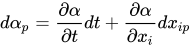






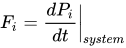


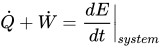

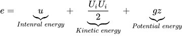

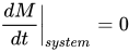




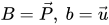












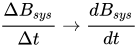

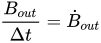
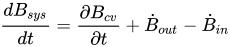









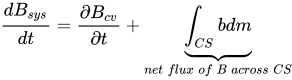

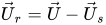











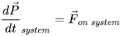
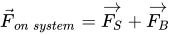
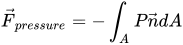
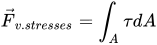





![{\displaystyle \displaystyle {\frac {dE}{dt}}_{system}=[{\dot {Q}}+{\dot {W}}]_{system}=[{\dot {Q}}+{\dot {W}}]_{cv}}](https://wikimedia.org/api/rest_v1/media/math/render/svg/53d98d9b1435500a0e7e2a680e39d51c37ec6106)
![{\displaystyle \displaystyle [{\dot {Q}}+{\dot {W}}]_{cv}={\frac {\partial }{\partial t}}\int _{cv}{e\rho dV}+\int _{cs}{e\rho {\vec {U}}\cdot {\vec {n}}dA}}](https://wikimedia.org/api/rest_v1/media/math/render/svg/a14d62b0ced65ed4d1cde67723f5ab31777e11c9)









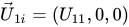

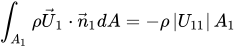



![{\displaystyle \displaystyle \int _{A_{2}}{\rho {\vec {U}}_{2}\cdot {\vec {n}}_{2}dA}=-\left[-\rho \left|U_{1}\right|A_{1}+{\dot {m}}_{3}-\rho Q_{4}\right]}](https://wikimedia.org/api/rest_v1/media/math/render/svg/041c07a9bc7dd38fdc4174c3eef414b73671b335)






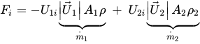



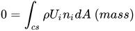

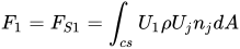












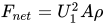



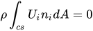


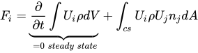















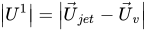
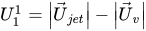




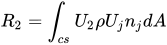


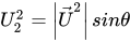
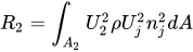
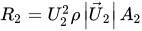
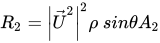

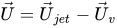



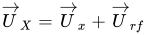

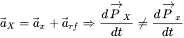
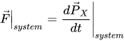

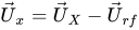


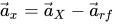


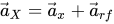
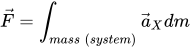
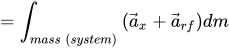










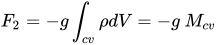






![{\displaystyle \displaystyle {\frac {\partial }{\partial t}}\left[\underbrace {\int _{CVI}{U_{2}\rho dV}} _{U_{2}=0\rightarrow =0}+\int _{CVII}{U_{2}\rho dV}\right]={\frac {\partial }{\partial t}}\int _{CVII}{U_{2}\rho dV}\approx 0}](https://wikimedia.org/api/rest_v1/media/math/render/svg/ee668e8eb095cc59b279da15cf892a47bf26c488)


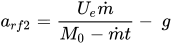




![{\displaystyle \displaystyle \left[{\dot {Q}}+{\dot {W}}\right]_{on\ system}=\left[{\dot {Q}}+{\dot {W}}\right]_{on\ cv}={\frac {\partial }{\partial t}}\int {e\rho \ dV}+\int _{cs}{e\rho {\vec {U}}\cdot {\vec {n}}dA}}](https://wikimedia.org/api/rest_v1/media/math/render/svg/9af4a72546078be9cc597e0c70a25299d4a87606)
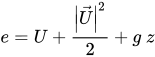






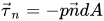

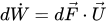










![{\displaystyle \displaystyle {\dot {Q}}=-{\dot {W}}_{shaft}+{\dot {m}}\left[h_{2}+{\frac {U_{2}^{2}}{2}}-h_{1}+\underbrace {g(z_{2}-z_{1})} _{=\ 0}\right]}](https://wikimedia.org/api/rest_v1/media/math/render/svg/33722aa4263638b6b2c0b494877751b1a93a055b)


![{\displaystyle \displaystyle {\dot {Q}}=-{\dot {W}}_{shaft}+{\dot {m}}\left[c_{p}(T_{2}-T_{1})+{\frac {U_{2}^{2}}{2}}\right]}](https://wikimedia.org/api/rest_v1/media/math/render/svg/63b9dc106739eb34f243f8b3838d3f69048120b1)


![{\displaystyle \displaystyle K={\dot {m}}\left[(u_{2}-u_{1})+\left({\frac {p_{2}}{\rho _{2}}}-{\frac {p_{1}}{\rho _{1}}}\right)+\left({\frac {{\vec {U}}_{2}^{2}}{2}}-{\frac {{\vec {U}}_{1}^{2}}{2}}\right)+g(z_{2}-z_{1})\right]}](https://wikimedia.org/api/rest_v1/media/math/render/svg/bf45ed0afe4c0680754abcac789524d6e0ef1dbf)




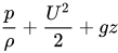


![{\displaystyle \displaystyle h_{loss}=\left[u_{2}-u_{1}-{\frac {\dot {Q}}{\dot {m}}}\right]{\frac {1}{g}}}](https://wikimedia.org/api/rest_v1/media/math/render/svg/3ea4dc98a083aad437b34ad5b7b18e09b379f9d9)



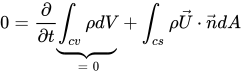

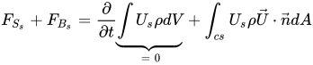

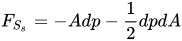








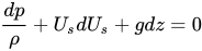

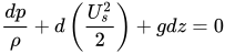

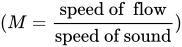


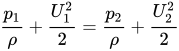


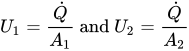
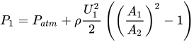
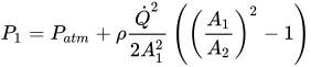
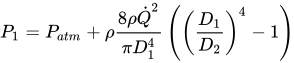





![{\displaystyle \displaystyle U_{2}^{2}\left[1-\left({\frac {A_{2}}{A_{1}}}\right)^{2}\right]=2gh}](https://wikimedia.org/api/rest_v1/media/math/render/svg/8f4f5e1790342fd2bdd3480c1f629ed503c89505)
![{\displaystyle \displaystyle U_{2}^{2}={\frac {2gh}{\left[1-\left({\frac {A_{2}}{A_{1}}}\right)^{2}\right]}}}](https://wikimedia.org/api/rest_v1/media/math/render/svg/adc836da27a09df149ef6584c4ec483dce5d8358)