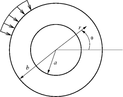
An elastic disk with a central circular hole
|
Under general loading, for the stresses and displacements to be single-valued and continuous, they must be periodic in
, e.g.,
.
An Airy stress function appropriate from this situation is
![{\displaystyle {\text{(83)}}\qquad \varphi =\sum _{n=0}^{\infty }f_{n}(r)\cos(n\theta )+\sum _{n=0}^{\infty }g_{n}(r)\sin(n\theta )}](https://wikimedia.org/api/rest_v1/media/math/render/svg/060072c015da073f1932cc9d5585ba50ad1d876f)
In the absence of body forces,
![{\displaystyle {\text{(84)}}\qquad \nabla ^{4}{\varphi }=\nabla ^{2}{(\nabla ^{2}{\varphi })}=0~;~~\nabla ^{2}{}=\left({\cfrac {\partial ^{2}}{\partial r^{2}}}+{\cfrac {1}{r}}{\cfrac {\partial }{\partial r}}+{\cfrac {1}{r^{2}}}{\cfrac {\partial ^{2}}{\partial \theta ^{2}}}\right)}](https://wikimedia.org/api/rest_v1/media/math/render/svg/dd09a302cce85777d45159fee265ab4a6ec24000)
Plug in
.
![{\displaystyle {\begin{aligned}\nabla ^{2}{\varphi }=&\sum _{n=0}^{\infty }\left[f_{n}^{''}(r)\cos(n\theta )+{\cfrac {1}{r}}f_{n}^{'}(r)\cos(n\theta )-{\cfrac {n^{2}}{r^{2}}}f_{n}(r)\cos(n\theta )\right]+\\&\sum _{n=0}^{\infty }\left[g_{n}^{''}(r)\sin(n\theta )+{\cfrac {1}{r}}g_{n}^{'}(r)\sin(n\theta )-{\cfrac {n^{2}}{r^{2}}}g_{n}(r)\sin(n\theta )\right]\qquad {\text{(85)}}\end{aligned}}}](https://wikimedia.org/api/rest_v1/media/math/render/svg/f0a4a16efc438da971bf8b10da293bb09a8ac069)
or,
![{\displaystyle {\text{(86)}}\qquad \nabla ^{2}{\varphi }=\sum _{n=0}^{\infty }F_{n}(r)\cos(n\theta )+\sum _{n=0}^{\infty }G_{n}(r)\sin(n\theta )}](https://wikimedia.org/api/rest_v1/media/math/render/svg/67c1e6377078023bc155c8ad2510d8b8edc1d5da)
Therefore,
![{\displaystyle {\begin{aligned}\nabla ^{4}{\varphi }=&\sum _{n=0}^{\infty }\left[F_{n}^{''}(r)\cos(n\theta )+{\cfrac {1}{r}}F_{n}^{'}(r)\cos(n\theta )-{\cfrac {n^{2}}{r^{2}}}F_{n}(r)\cos(n\theta )\right]+\\&\sum _{n=0}^{\infty }\left[G_{n}^{''}(r)\sin(n\theta )+{\cfrac {1}{r}}G_{n}^{'}(r)\sin(n\theta )-{\cfrac {n^{2}}{r^{2}}}G_{n}(r)\sin(n\theta )\right]\qquad {\text{(87)}}\end{aligned}}}](https://wikimedia.org/api/rest_v1/media/math/render/svg/fd8143d7cc3c8acf0d977768fee305c35a857ad8)
To satisfy the compatibility condition
, we need
![{\displaystyle {\begin{aligned}{\text{(88)}}\qquad F_{n}^{''}(r)+{\cfrac {1}{r}}F_{n}^{'}(r)-{\cfrac {n^{2}}{r^{2}}}F_{n}(r)&=0\\{\text{(89)}}\qquad G_{n}^{''}(r)+{\cfrac {1}{r}}G_{n}^{'}(r)-{\cfrac {n^{2}}{r^{2}}}G_{n}(r)&=0\end{aligned}}}](https://wikimedia.org/api/rest_v1/media/math/render/svg/d4ccce90a6b362275aaea57c3bf54ba8d6c12f0d)
The general solution of these Euler-Cauchy type equations is
![{\displaystyle {\begin{aligned}{\text{(90)}}\qquad F_{n}(r)&=A_{1}r^{n}+B_{1}r^{-n}\\{\text{(91)}}\qquad G_{n}(r)&=C_{1}r^{n}+D_{1}r^{-n}\end{aligned}}}](https://wikimedia.org/api/rest_v1/media/math/render/svg/a2952c5c35f44bd8f25db6087c03ee502be71520)
We can use either to determine
. Thus,
![{\displaystyle {\text{(92)}}\qquad f_{n}^{''}(r)+{\cfrac {1}{r}}f_{n}^{'}(r)-{\cfrac {n^{2}}{r^{2}}}f_{n}(r)=A_{1}r^{n}+B_{1}r^{-n}}](https://wikimedia.org/api/rest_v1/media/math/render/svg/503d27621e9a753917953ae8b39c0d90dbb8eb2d)
or,
![{\displaystyle {\text{(93)}}\qquad r^{2}f_{n}^{''}(r)+rf_{n}^{'}(r)-n^{2}f_{n}(r)=A_{1}r^{n+2}+B_{1}r^{-n+2}}](https://wikimedia.org/api/rest_v1/media/math/render/svg/0980bdb5511a1558cfab1a88370784b213569fce)
The homogeneous and particular solutions of this equation are
![{\displaystyle {\begin{aligned}{\text{(94)}}\qquad f_{n}^{h}(r)&=A_{2}r^{n}+B_{2}r^{-n}\\{\text{(95)}}\qquad f_{n}^{p}(r)&=A_{1}r^{n+2}+B_{1}r^{-n+2}\end{aligned}}}](https://wikimedia.org/api/rest_v1/media/math/render/svg/ca422afd2e0f1c110b0af84070f82e64a41848ed)
Hence, the general solution is
![{\displaystyle {\text{(96)}}\qquad f_{n}(r)=A_{1}r^{n+2}+B_{1}r^{-n+2}+A_{2}r^{n}+B_{2}r^{-n}}](https://wikimedia.org/api/rest_v1/media/math/render/svg/a52013dd83448578f330789bf28cf9e413f6d1aa)
This form is valid for
. If
, alternative forms are obtained. Thus,
![{\displaystyle {\begin{aligned}{\text{(97)}}\qquad f_{0}(r)&=A_{O}r^{2}+B_{0}r^{2}\ln r+C_{0}+D_{0}\ln r\\{\text{(98)}}\qquad f_{1}(r)&=A_{1}r^{3}+B_{1}r+C_{1}r\ln r+D_{1}r^{-1}\\{\text{(99)}}\qquad f_{n}(r)&=A_{n}r^{n+2}+B_{n}r^{n}+C_{n}r^{-n+2}+D_{n}r^{-n}~,~~n>1\end{aligned}}}](https://wikimedia.org/api/rest_v1/media/math/render/svg/740f91c6cdd8bafc5661ffcda43fcf0436d7eaee)
Terms in
are chosen according to the specific problem of interest.
- at
![{\displaystyle r=a}](https://wikimedia.org/api/rest_v1/media/math/render/svg/e193cdce556664593cd0a8347617f5284d0364c9)
![{\displaystyle {\text{(100)}}\qquad \sigma _{rr}=T_{1}(\theta )~,~~\sigma _{r\theta }=T_{2}(\theta )}](https://wikimedia.org/api/rest_v1/media/math/render/svg/010de81479f5040c090159c542c898a669c55498)
- at
![{\displaystyle r=b}](https://wikimedia.org/api/rest_v1/media/math/render/svg/1214af636c70a8359956e08b2c20c64b59c6071a)
![{\displaystyle {\text{(101)}}\qquad \sigma _{rr}=T_{3}(\theta )~,~~\sigma _{r\theta }=T_{4}(\theta )}](https://wikimedia.org/api/rest_v1/media/math/render/svg/668f1cdb0abcf286754629ecbe6f5a60bb6137e5)
Express
in Fourier series form.
![{\displaystyle {\text{(102)}}\qquad T_{i}(\theta )=\sum _{n=0}^{\infty }A_{ni}\cos(n\theta )+\sum _{n=0}^{\infty }B_{ni}\sin(n\theta )~,~~i=1,2,3,4}](https://wikimedia.org/api/rest_v1/media/math/render/svg/57db714a765c53606fc83624b2b0ca83f17862c9)
Terms in
are chosen according to the specific problem of interest.