University of Florida/Eml4507/s13 Report 4 Team 7

Problem 1

On our honor, we did this assignment on our own, without looking at the solutions in previous semesters or other online solutions.

Find

Find the eigenvector x₂ corresponding to the eigenvalue λ₂ for the spring-mass-damper system on p. 53-13. Plot and comment on this mode shape. Verify that the eigenvectors are orthogonal to each other.

Given

The spring-mass-damper system shown on p. 53-13.

Solution

I=identity matrix

Need to find an eigenvector where



By solving this matrix, and setting x₁=1, then two equations are created.

k₁+k₂-γ₂-k₂x₂=0

and

-k₂+(k₂+k₃-γ₂)x₂=0

Therefore,

x₂=(γ₂-k₁)/(k₃-γ₂)

Two eigenvectors are orthogonal if their dot product is 0.

The dot product of x₁ and x₂ however is not 0, therefore they are not orthogonal.

Problem 2

On our honor, we did this assignment on our own, without looking at the solutions in previous semesters or other online solutions.

Find

Find, plot and compare the eigenvectors.
Compare the mode shapes using two different assumptions.
Animate each format in the given sine wave.

Given

$\mathbf {|x_{1}x_{2}|} ={\begin{bmatrix}x_{11}&x_{12}\\x_{21}&x_{22}\\\end{bmatrix}}$

(2.1)

Solve for the eigenvectors under two differing assumptions:

$x_{11}=x_{12}=1$ and $x_{21}=x_{22}=1$

(2.2)

Mode shapes were plotted according to $y=x_{i}sin(w_{i}t)$

where $w_{i}t$ is the circular frequency, $w_{i}t={\sqrt {(}}l_{i})$

$l_{1}$ is the eigenvalue $4+{\sqrt {(}}5)$. $l_{2}$ is the eigenvalue $4-{\sqrt {(}}5)$.

Solution

Firstly, the eigenvectors must be found. The $x_{21}=1$ assumption is in effect. These values were found with $l_{1}=4+{\sqrt {5}}$

${\begin{bmatrix}k-yI\\\end{bmatrix}}X={\begin{bmatrix}0\\\end{bmatrix}}$

(2.3)

${\begin{bmatrix}-1+{\sqrt {(}}5)&-2\\-2&1+{\sqrt {(}}5)\\\end{bmatrix}}{\begin{bmatrix}x_{1}\\1\\\end{bmatrix}}={\begin{bmatrix}0\\0\\\end{bmatrix}}$

(2.4)

$-2x_{1}+1+{\sqrt {(}}5)=0$ $x_{1}=(1+{\sqrt {5}})/2$

(2.5)

and now, The $x_{11}=1$ assumption is in effect.

${\begin{bmatrix}k-yI\\\end{bmatrix}}X={\begin{bmatrix}0\\\end{bmatrix}}$

(2.6)

${\begin{bmatrix}-1+{\sqrt {(}}5)&-2\\-2&1+{\sqrt {(}}5)\\\end{bmatrix}}{\begin{bmatrix}1\\x_{2}\\\end{bmatrix}}={\begin{bmatrix}0\\0\\\end{bmatrix}}$

(2.7)

$-1+sqrt{5}-2x_{2}=0$ $x_{2}=(-1+{\sqrt {5}})/2$

(2.8)

and now, The $x_{21}=1$ assumption is in effect. These values were found with $l_{2}=4-{\sqrt {5}}$

${\begin{bmatrix}k-yI\\\end{bmatrix}}X={\begin{bmatrix}0\\\end{bmatrix}}$

(2.9)

${\begin{bmatrix}-1-{\sqrt {(}}5)&-2\\-2&1-{\sqrt {(}}5)\\\end{bmatrix}}{\begin{bmatrix}x_{1}\\1\\\end{bmatrix}}={\begin{bmatrix}0\\0\\\end{bmatrix}}$

(2.10)

$-2x_{1}+1-{\sqrt {(}}5)=0$ $x_{1}=(1-{\sqrt {5}})/2$

(2.11)

and now, The $x_{11}=1$ assumption is in effect.

${\begin{bmatrix}k-yI\\\end{bmatrix}}X={\begin{bmatrix}0\\\end{bmatrix}}$

(2.12)

${\begin{bmatrix}-1-{\sqrt {(}}5)&-2\\-2&1-{\sqrt {(}}5)\\\end{bmatrix}}{\begin{bmatrix}1\\x_{2}\\\end{bmatrix}}={\begin{bmatrix}0\\0\\\end{bmatrix}}$

(2.13)

$-1-sqrt{5}-2x_{2}=0$ $x_{2}=(-1-{\sqrt {5}})/2$

(2.14)

Now with these values solved for, construct the eigenvectors:

$x_{1}={\begin{bmatrix}{1+{\sqrt {5}}}/2&{1-{\sqrt {5}}}/2\\1&1\\\end{bmatrix}}$ and $x_{2}={\begin{bmatrix}1&1\\{-1+{\sqrt {5}}}/2&{-1-{\sqrt {5}}}/2\\\end{bmatrix}}$ Using this MATLAB code, each mode was plotted, and comparisons can be made. M1 =[ 1.618 -.618; 1 1; ]; quiver(0,0,M1(1,1),M1(2,1)); hold on; quiver(0,0,M1(1,2),M1(2,2)); M2 =[ 1 1; 0.618 -1.618; ]; quiver(0,0,M2(1,1),M2(2,1)); hold on; quiver(0,0,M2(1,2),M2(2,2)); %% Sine wave: x1lambda1 = [1.618; 1;]; x2lambda1 = [-.618; 1;]; x1lambda2 = [1; .618;]; x2lambda2 = [1; -1.618;]; omega1 = sqrt(4 - sqrt(5)); omega2 = sqrt(4 + sqrt(5)); t = 0:pi/30:4*pi; x1 = x1lambda1*sin(omega1*t); x2 = x2lambda1*sin(omega1*t); x3 = x1lambda2*sin(omega2*t); x4 = x2lambda2*sin(omega2*t); figure; %mode 1 plot(t,x1); plot(t,x2); %mode 2 plot(t,x3); plot(t,x4);

Mode 1

Mode 2

Mode 1 and Mode 2 have the same angle between vectors. Mode 2 is flipped over the $y=x$ line.

Modes animated according to sine graphs:

Mode 1 Animation

Mode 2 Animation

Problem 3

On our honor, we did this assignment on our own, without looking at the solutions in previous semesters or other online solutions.

Find

Discuss the computational efficiency of Method 1 (root sum squared method) vs. Method 2 (transformation matrix method)

Solution

The root sum square method is less useful than the transformation matrix method because the Transformation Matrix method can be used for all other elements where as the root sum square method can be used only for the bar elements as stated in MTG 23.

The overall forces in Method 1 are found by summing the squares of each component (x,y,z) and then taking the square root of that sum for the overall force and direction of the 2D or 3D system.

Both methods use the relation that F=kd but method two goes through more steps to allow a better way for finding the stresses in each element together instead of individually.

In the end both methods will give the same answer but Method 2 is more useful when more elements are involved.

Problem 4

On our honor, we did this assignment on our own, without looking at the solutions in previous semesters or other online solutions.

Find

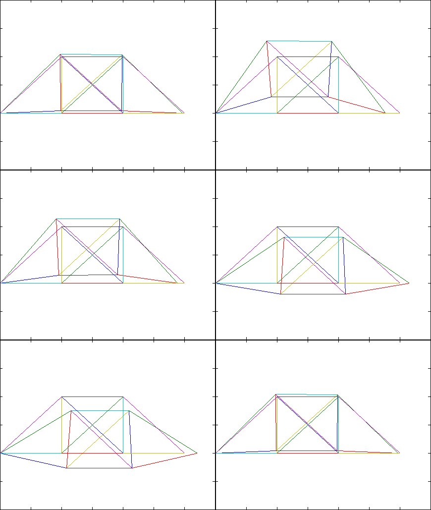
The Lowest 3 eigenpairs $(\omega _{j},\phi _{j})forj=1,2,3$ and plot the 3 lowest mode shapes in a gif image.

Given

Figure 6.1: 25 member truss with L=0.3 m

$E=100GPa,A=1.0cm^{2},L=0.3m,\rho =5000{\frac {kg}{m^{3}}}$

Solution

 
%GIVENS
L=0.3;
E=100e9;
A=1e-4;
rho=5000;
ep=[E A];

%ELEMENT DOF
Edof=zeros(25,5);
for i=1:6
    j=2*(i-1);
    Edof(i,:)=[i,1+j,2+j,3+j,4+j];
end
for i=7:12
    j=2*(i+1);
    Edof(i,:)=[i,j-1,j,j+1,j+2];
end
for i=13:19
    j=2*(i-13);
    Edof(i,:)=[i,1+j,2+j,15+j,16+j];
end
for i=20:25
    j=2*(i-20);
    Edof(i,:)=[i,1+j,2+j,17+j,18+j];
end

%COORDINATES
ex=zeros(14,2);
ey=zeros(14,2);
for i=1:25
    if i<7
        ex(i,:)=[L*(i-1),L*i];
        ey(i,:)=[0,0];
    elseif i>6&&i<13
        ex(i,:)=[L*(i-7),L*(i-6)];
        ey(i,:)=[L,L];
    elseif i>12&&i<20
        ex(i,:)=[L*(i-13),L*(i-13)];
        ey(i,:)=[0,L];
    else
        ex(i,:)=[L*(i-20),L*(i-19)];
        ey(i,:)=[0,L];
    end
end

%STIFFNESS MATRIX
K=zeros(28);
M=zeros(28);
for i=1:25
    E=ep(1);A=ep(2);
    xt=ex(i,2)-ex(i,1);
    yt=ey(i,2)-ey(i,1);
    L=sqrt(xt^2+yt^2);
    l=xt/L; m=yt/L;
    ke=E*A/L*[l^2 l*m -l^2 -l*m;
              l*m m^2 -l*m -m^2;
              -l^2 -l*m l^2 l*m;
              -l*m -m^2 l*m m^2;];
    m=L*A*rho;
    me=[m/2 0 0 0;
        0 m/2 0 0;
        0 0 m/2 0;
        0 0 0 m/2];
    edoft=Edof(i,2:5);
    K(edoft,edoft)=K(edoft,edoft)+ke;
    M(edoft,edoft)=M(edoft,edoft)+me;
end

nd=size(K,1);
fdof=[1:nd]';
b=[1 15 16]';
fdof(b(:))=[];
[X,D]=eig(K(fdof,fdof),M(fdof,fdof));
nfdof=size(X,1);
eigenval=diag(D);
eigenvec=zeros(nd,nfdof);
eigenvec(fdof,:)=X;

eigenval1=eigenval(1)
eigenvec1=eigenvec(:,1)
eigenval2=eigenval(2)
eigenvec2=eigenvec(:,2)
eigenval3=eigenval(3)
eigenvec3=eigenvec(:,3)

t=Edof(:,2:5);
eignmode=eigenvec(:,2);
for i = 1:25
    Edb(i,1:4)=eignmode(t(i,:))';
end
       
eldraw2(ex,ey)

The resulting egienpairs are:

$\displaystyle {\begin{aligned}&\omega _{1}=1.6890\times 10^{5}\phi _{1}={\begin{bmatrix}0\\-0.0082\\-0.0279\\-0.0757\\-0.0479\\-0.1982\\-0.0605\\-0.3581\\-0.0670\\-0.5384\\-0.0690\\-0.7244\\-0.0690\\-0.9052\\0\\0\\0.0364\\-0.0677\\0.0645\\-0.1906\\0.0847\\-0.3514\\0.0974\\-0.5332\\0.1038\\-0.7213\\0.1058\\-0.9045\end{bmatrix}}\\&\omega _{2}=2.6676\times 10^{6}\phi _{2}={\begin{bmatrix}0\\-0.0745\\0.0227\\-0.4176\\0.0973\\-0.6512\\0.1884\\-0.6252\\0.2603\\-0.3137\\0.2941\\0.1825\\0.2976\\0.6937\\0\\0\\0.0732\\-0.3541\\0.0714\\-0.6149\\0.0153\\-0.6228\\-0.0603\\-0.3368\\-0.1201\\0.1553\\-0.1455\\0.6853\end{bmatrix}}\\&\omega _{3}=7.0219\times 10^{6}\phi _{3}={\begin{bmatrix}0\\-0.0352\\-0.2178\\-0.0416\\-0.3907\\-0.1023\\-0.5191\\-0.1283\\-0.6115\\-0.0751\\-0.6722\\0.0253\\-0.6941\\0.0971\\0\\0\\-0.1204\\-0.0089\\-0.2656\\-0.0780\\-0.4221\\-0.1195\\-0.5663\\-0.0809\\-0.6710\\0.0154\\-0.7178\\0.0940\end{bmatrix}}\\\end{aligned}}$

Combining the images into a gif results in the following

Figure 4.2: 25 first 3 eigenmodes

Contributing Team Members

Problem Assignments
Problem #	Solved & Typed by	Reviewed by
1	Kristin Howe	All
2	Joshua Plicque	All
3	Brandon Wright	All
4	Matthew Gidel,Spencer Herran	All

On our honor, we did this assignment on our own, without looking at the solutions in previous semesters or other online solutions.