Plasmas/Plasma objects/Coronal clouds

A coronal cloud is a cloud, or cloud-like, natural astronomical entity, composed of plasmas and usually associated with a star or other astronomical object where the temperature is such that X-rays are emitted. While small coronal clouds are above the photosphere of many different visual spectral type stars, others occupy parts of the interstellar medium (ISM), extending sometimes millions of kilometers into space, or thousands of light-years, depending on the size of the associated object such as a galaxy.
Astronomy[edit | edit source]
Once an entity, source, or object [such as a corona or coronal cloud] has been detected as emitting, reflecting, absorbing, transmitting, or fluorescing radiation, it may be necessary to determine what the mechanism is. Usually this information provides understanding of the same entity, source, or object.
The coronal cloud in close proximity to the Sun also emits X-rays that produce visual fluorescence from gases in a comet's coma and tail. Is the Sun an entity controlling the sky or is it the coronal cloud surrounding the Sun?
Radiation[edit | edit source]
"This energy [1032 to 1033 ergs] appears in the form of electromagnetic radiation over the entire spectrum from γ-rays to radio burst, in fast electrons and nuclei up to relativistic energies, in the creation of a hot coronal cloud, and in large-scale mass motions including the ejections of material from the Sun."[1]
Planetary sciences[edit | edit source]

"Auroras are produced by solar storms that eject clouds of energetic charged particles. These particles are deflected when they encounter the Earth’s magnetic field, but in the process large electric voltages are created. Electrons trapped in the Earth’s magnetic field are accelerated by these voltages and spiral along the magnetic field into the polar regions. There they collide with atoms high in the atmosphere and emit X-rays".[2]
In the image at right are bright X-ray arcs suggestive of the presence of a coronal cloud. The images are superimposed on a simulated image of the Earth. The color code represents brightness, maximum in red. Distance from the North pole to the black circle is 3,340 km (2,080 mi). Observation dates: 10 pointings between December 16, 2003 and April 13, 2004.
Coronal cloud theory[edit | edit source]
Coronal loops have become very important when trying to understand the current coronal heating problem. Coronal loops are highly radiating sources of plasma and therefore easy to observe by instruments such as TRACE; they are highly observable laboratories to study phenomena such as solar oscillations, wave activity and nanoflares. However, it remains difficult to find a solution to the coronal heating problem as these structures are being observed remotely, where many ambiguities are present (i.e. radiation contributions along the LOS). In-situ measurements are required before a definitive answer can be arrived at, but due to the high plasma temperatures in the corona, in-situ measurements are impossible (at least for the time being). The next mission of the Nasa Solar Probe Plus will approach the Sun very closely allowing more direct observations.
The coronal heating problem in solar physics relates to the question of why the temperature of the Sun's corona is millions of kelvin higher than that of the surface. The high temperatures require energy to be carried from the solar interior to the corona by non-thermal processes, because the second law of thermodynamics prevents heat from flowing directly from the solar photosphere, or surface, at about 5800 K, to the much hotter corona at about 1 to 3 MK (parts of the corona can even reach 10 MK).
The thin region of temperature increase from the chromosphere to the corona is known as the transition region and can range from tens to hundreds of kilometers thick. An analogy of this would be a light bulb heating the air surrounding it hotter than its glass surface. The second law of thermodynamics would be broken.
The amount of power required to heat the solar corona can easily be calculated as the difference between coronal radiative losses and heating by thermal conduction toward the chromosphere through the transition region. It is about 1 kilowatt for every square meter of surface area on the Sun, or 1/40000 of the amount of light energy that escapes the Sun.
Many coronal heating theories have been proposed,[3] but two theories have remained as the most likely candidates, wave heating and magnetic reconnection (or nanoflares).[4] Through most of the past 50 years, neither theory has been able to account for the extreme coronal temperatures.
| Heating Models | ||
|---|---|---|
| Hydrodynamic | Magnetic | |
|
DC (reconnection) | AC (waves) |
|
| |
| Not our Sun! | Competing theories | |
Magnetic reconnection is hypothesized to be the mechanism behind solar flares, the largest explosions in our solar system. Furthermore, the surface of the Sun is covered with millions of small magnetized regions 50–1,000 km across. These small magnetic poles are buffeted and churned by the constant granulation. The magnetic field in the solar corona must undergo nearly constant reconnection to match the motion of this "magnetic carpet", so the energy released by the reconnection is a natural candidate for the coronal heat, perhaps as a series of "microflares" that individually provide very little energy but together account for the required energy.
Def. the "luminous plasma atmosphere of the Sun or other star, extending millions of kilometres into space, most easily seen during a total solar eclipse"[5] is called a corona, or stellar corona.
Entities[edit | edit source]
Historical evidence exists for the phrase "coronal cloud" with respect to "a cloud, or cloud-like, natural astronomical entity, composed of plasmas, at least hot enough to emit X-rays". For now this may serve as a working definition.
Def. a cloud, or cloud-like, natural astronomical entity, composed of plasmas at least hot enough to emit X-rays is called a coronal cloud.
The idea that nanoflares might heat the corona was put forward by Eugene Parker in the 1980s but is still controversial. In particular, ultraviolet telescopes such as TRACE and SOHO/EIT can observe individual micro-flares as small brightenings in extreme ultraviolet light,[6] but there seem to be too few of these small events to account for the energy released into the corona. The additional energy not accounted for could be made up by wave energy, or by gradual magnetic reconnection that releases energy more smoothly than micro-flares and therefore doesn't appear well in the TRACE data. Variations on the micro-flare hypothesis use other mechanisms to stress the magnetic field or to release the energy, and are a subject of active research in 2005.
Sources[edit | edit source]
As of December 5, 2011, "Voyager 1 is about ... 18 billion kilometers ... from the [S]un [but] the direction of the magnetic field lines has not changed, indicating Voyager is still within the heliosphere ... the outward speed of the solar wind had diminished to zero in April 2010 ... inward pressure from interstellar space is compacting [the magnetic field] ... Voyager has detected a 100-fold increase in the intensity of high-energy electrons from elsewhere in the galaxy diffusing into our solar system from outside ... [while] the [solar] wind even blows back at us."[7]
"[P]ower spectra intrinsic to the source can be severely attenuated at high frequencies by scattering in a hot coronal cloud with the amount of attenuation depending on optical depth and cloud radius."[8] A Z source is a low-mass X-ray binary exhibiting a Z-type X-ray intensity profile, as resembling the letter "Z".
Objects[edit | edit source]
"Coronal clouds are irregular objects suspended in the corona with matter streaming out of them into nearby active regions."[9]
"Objects identified as X-ray bright points show complex resolved structure; but a new class of bright points connected with satellite polarity was smaller and more complex."[10]
"The object of interest here is the bright streamer in the southeast quadrant."[11]
Continua[edit | edit source]
"High time resolution videotapes of the blue continuum show no fluctuations faster than a few seconds."[12]
"All parameters seem to have broad or unimodal distributions, suggesting that flares and CMEs form a continuum with the same underlying physics."[13]
"At the NIXT wavelength, the opacity will be dominated by Lyman-continuum absorption of neutral H and He."[10]
"The peak continuum intensity was always at the loop tops."[14]
Bands[edit | edit source]
"In the L-band, a diffuse single source is observed. It is located between the two ribbons observed in the higher-energy bands."[15]
"They also roughly match the off-band Hα images, ie, the region of broad Hα profile."[12]
"A flare mode normally triggers at about the C2 level, 2 x 10³ ergs (cm2 sec)-1 in the 1-8 A band."[16]
Backgrounds[edit | edit source]
For coronal cloud observations of the Large Magellanic Cloud, "[b]ackground spectra were obtained from observations of the Lockman Hole."[17]
"With longer exposures and instruments whose stray light background is low, it is probable that there would be observed at least as many emission lines per nanometre as there are Fraunhofer lines per nanometre at longer wavelengths."[18]
"In between is an irregular continuous background field of about 0.05 gauss, which Zhang and Zirin recently found had a net polarity opposite the dominant field in that hemisphere."[19]
Temperatures[edit | edit source]
The high temperature of the coronal cloud gives it unusual spectral features. These features have been traced to highly ionized atoms of elements such as iron which indicate a plasma's temperature in excess of 106 Kelvin (MK).
Although a coronal cloud (as part or all of a stellar or galactic corona) is usually "filled with high-temperature plasma at temperatures of T ≈ 1–2 (MK), ... [h]ot active regions and postflare loops have plasma temperatures of T ≈ 2–40 MK."[20]
Coronal heating[edit | edit source]
"The photosphere of the Sun has an effective temperature of 5,570 K[21] yet its corona has an average temperature of 1–2 x 10⁶ K.[22] However, the hottest regions are 8–20 x 106 K.[22] The high temperature of the corona shows that it is heated by something other than direct heat conduction from the photosphere.[23]
It is thought that the energy necessary to heat the corona is provided by turbulent motion in the convection zone below the photosphere, and two main mechanisms have been proposed to explain coronal heating.[22] The first is wave heating, in which sound, gravitational or magnetohydrodynamic waves are produced by turbulence in the convection zone.[22] These waves travel upward and dissipate in the corona, depositing their energy in the ambient gas in the form of heat.[24] The other is magnetic heating, in which magnetic energy is continuously built up by photospheric motion and released through magnetic reconnection in the form of large solar flares and myriad similar but smaller events—nanoflares.[25]
Currently, it is unclear whether waves are an efficient heating mechanism. All waves except Alfvén waves have been found to dissipate or refract before reaching the corona.[26] In addition, Alfvén waves do not easily dissipate in the corona. Current research focus has therefore shifted towards flare heating mechanisms.[22]"[27]
Meteors[edit | edit source]

A magnetic cloud is a transient event observed in the solar wind. It was defined in 1981 by Burlaga et al. 1981 as a region of enhanced magnetic field strength, smooth rotation of the magnetic field vector and low proton temperature [28]. Magnetic clouds are a possible manifestation of a Coronal Mass Ejection (CME). The association between CMEs and magnetic clouds was made by Burlaga et al. in 1982 when a magnetic cloud was observed by Helios-1 two days after being observed by SMM[29]. However, because observations near Earth are usually done by a single spacecraft, many CMEs are not seen as being associated with magnetic clouds. The typical structure observed for a fast CME by a satellite such as ACE is a fast-mode shock wave followed by a dense (and hot) sheath of plasma (the downstream region of the shock) and a magnetic cloud.
Other signatures of magnetic clouds are now used in addition to the one described above: among other, bidirectional superthermal electrons, unusual charge state or abundance of iron, helium, carbon and/or oxygen. The typical time for a magnetic cloud to move past a satellite at the L1 point is 1 day corresponding to a radius of 0.15 AU with a typical speed of 450 km s−1 and magnetic field strength of 20 nT [30]
Def. a "massive burst of solar wind, other light isotope plasma, and magnetic fields rising above the solar corona or being released into space"[31] is called a coronal mass ejection (CME).
An explosive limb flare occurred above 30,000 km in the corona of the Sun.[32] "So the aftermath of the flare explosion, usually visible in disk pictures as extensive Hα brightening, but hidden from us in this case, was seen by the ionosphere as an intense flux of ionizing radiation from the coronal cloud created by the explosion."[32] "The November 20, 1960, event is very similar to that of February 10, 1956, which was observed at Sacramento Peak. A bright ball appears above the surface, grows in size and Hα brightness, and explodes upward and outward."[32] "The great breadth and intensity of the Hα emission from the suspended ball at 2013 U.T. testify to the large amount of energy stored there, as no corresponding macroscopic motion was observed until the explosion at 2023 U.T."[32] "[T]he great energy of the preflare cloud was released into the corona by the explosion of 2023 U.T., and Hα radiation disappeared by 2035 U.T."[32]
"On 16 June 1972, the Naval Research Laboratory's coronagraph aboard OSO-7 tracked a huge coronal cloud moving outward from the Sun."[11]
A coronal mass ejection (CME) is an ejected plasma consisting primarily of electrons and protons (in addition to small quantities of heavier elements such as helium, oxygen, and iron), plus the entraining coronal closed magnetic field regions. Evolution of these closed magnetic structures in response to various photospheric motions over different time scales (convection, differential rotation, meridional circulation) somehow leads to the CME.[33] Small-scale energetic signatures such as plasma heating (observed as compact soft X-ray brightening) may be indicative of impending CMEs.
The soft X-ray sigmoid (an S-shaped intensity of soft X-rays) is an observational manifestation of the connection between coronal structure and CME production.[33]
"Relating the sigmoids at X-ray (and other) wavelengths to magnetic structures and current systems in the solar atmosphere is the key to understanding their relationship to CMEs."[33]
Cosmic rays[edit | edit source]
"[C]oronal magnetic bottles, produced by flares, [may] serve as temporary traps for solar cosmic rays ... It is the expansion of these bottles at velocities of 300–500 km/s which allows fast azimuthal propagation of solar cosmic rays independent of energy. A coronagraph on Os 7 observed a coronal cloud which was associated with bifurcation of the underlying coronal structure."[34]
Neutrons[edit | edit source]
"The neutrons are produced by the energetic protons interacting with a number of different nuclei."[1]
Protons[edit | edit source]
"On 16 June 1972, the Naval Research Laboratory's coronagraph aboard OSO-7 tracked a huge coronal cloud moving outward from the Sun. ... This event is of great interest in its own right because it is the probable source of the solar proton event (Solar-Geophysical Data, NOAA Boulder) and shock-produced interplanetary scintillations (Dennison, 1972) which began early on 16 June."[11]
Electrons[edit | edit source]
"The density of the coronal cloud deduced in this case is about 2 x 10¹¹ electrons per cubic centimeter."[35]
Positrons[edit | edit source]
"On the basis of spectroscopic observations, the leading models of the X-ray continuum production are based on a hot, Comptonizing electron or electron-positron pair corona close to the black hole."[36]
Neutrinos[edit | edit source]

"The highest flux of solar neutrinos come directly from the proton-proton interaction, and have a low energy, up to 400 keV. There are also several other significant production mechanisms, with energies up to 18 MeV. [37]"[38]
"The parts of the Sun above the photosphere are referred to collectively as the solar atmosphere.[39]"[40]
"Neutrinos can be produced by energetic protons accelerated in solar magnetic fields. Such protons produce pions, and therefore muons, hence also neutrinos as a decay product, in the solar atmosphere."[41]
"Energetic protons in the solar corona could explain Figure 2 only if (1) they tap a substantial fraction of the entire energy generated in the corona, (2) the energy generated in the corona is at least 3 times what has been deduced from the observations, (3) the vast majority of energetic protons do not escape the Sun, (4) the proton energy spectrum is unusually hard (p0 = 300 MeV c-1, and (5) the sign of the variation is opposite to what one would predict. As the likelihood of all of these conditions being fulfilled seems extremely small, we do not believe that neutrinos produced by energetic protons in the solar atmosphere contribute significantly to the neutrino capture in the 37Cl experiment."[41]
Gamma rays[edit | edit source]
"The 2.2 MeV line is formed in the reaction which synthesizes deuterium: 1H(n,γ)2H ... The line has been observed in a number of solar flares by the SMM, Hinotori and Prognoz satellites".[42]
"The 2.2-MeV line fluence throughout the [May 24, 1990] flare was 345 ± 6 photons/cm2, which corresponds to the observed synthesis of over 3 tons [some ~3.3 metric tons] of deuterium on the solar surface."[42]
"Surface fusion is no longer bizarre since the 2.2 MeV gamma ray line of the P(n,γ)D reaction was observed[42] during the solar flare of May 24 1990."[43]
"[M]ost of the sun’s fusion must occur near the surface rather than the core."[43]
X-rays[edit | edit source]
"The origin of all observed astronomical X-ray sources is in, near to, or associated with a coronal cloud or gas at coronal cloud temperatures for however long or brief a period."[44]
Ultraviolets[edit | edit source]

"One of the fastest CMEs in years was captured by the STEREO COR1 telescopes on August 1, 2010. ... This CME is seen to be heading towards Earth at speeds well over 1000 kilometers per second."[45]
"On August 1st, almost the entire Earth-facing side of the sun erupted in a tumult of activity. There was a C3-class solar flare, a solar tsunami, multiple filaments of magnetism lifting off the stellar surface, large-scale shaking of the solar corona, radio bursts, a coronal mass ejection and more. This extreme ultraviolet snapshot [at right] from the Solar Dynamics Observatory (SDO) shows the sun's northern hemisphere in mid-eruption. Different colors in the image represent different gas temperatures ranging from ~1 to 2 million degrees K."[45]
Opticals[edit | edit source]

"The Pleiades star cluster is one of the jewels of the northern sky. To the unaided eye it appears as an alluring group of stars in the constellation Taurus, while telescopic views reveal cluster stars surrounded by delicate blue wisps of dust-reflected starlight. To the X-ray telescopes on board the orbiting ROSAT observatory, the cluster also presents an impressive, but slightly altered, appearance. This false color image [at right] was produced from ROSAT observations by translating different X-ray energy bands to visual colors - the lowest energies are shown in red, medium in green, and highest energies in blue. (The green boxes mark the position of the seven brightest visual stars.) The Pleiades stars seen in X-rays have extremely hot, tenuous outer atmospheres called coronas and the range of colors corresponds to different coronal temperatures."[46]
Visuals[edit | edit source]

"NASA gave people a front row seat to today's total solar eclipse, thanks to a partnership with the University of California at Berkeley and the Exploratorium. A streaming webcast brought the eclipse -- visible along a path from South America to Africa to Asia -- to schools and museums and computer desktops worldwide. ... The sun's corona, or outer atmosphere, is visible during totality -- when the sun is totally obscured by the [M]oon's shadow."[47]
Violets[edit | edit source]
Calcium has a line occurring in the solar corona at 408.63 nm of Ca XIII.[48]
Iron has a line occurring in the solar corona in the violet at 398.69 nm of Fe XI.[48]
Nickel has three emission lines occurring in the solar corona at 380.08 nm of Ni XIII and 423.14 nm and 431.1 of Ni XII.[48]
Blues[edit | edit source]
"[B]ound electrons in the corona [may be] scattering blue light according to RAYLEIGH'S law ... [The scattering coefficients and the intensities scattered] for blue and yellow light are in the proportion 37/11 = 3,36 [thus] the scattering must be due to bound electrons, belonging to ions or atoms."[49]
The continuous spectrum of the corona may result from the "[s]cattering of the photospheric light by the electrons in the corona ["by emission of the corona itself due to recombinations"] [or by] [t]he emission and the "scattering" in the corona ... described as one single process".[49]
"[T]he corona is supposed to be composed of electrons and positive ions, due to ejection from the photosphere".[49]
Sun[edit | edit source]

"Magnetic clouds represent about one third of ejecta observed by satellites at Earth. Other types of ejecta are multiple-magnetic cloud events (a single structure with multiple subclouds distinguishable)[50][51] and complex ejecta, which can be the result of the interaction of multiple CMEs."[52]
"Observations of the Hanle effect have revealed the existence of small-scale ‘hidden’ magnetic flux on the quiet Sun. The magnetic-energy density of this hidden flux is much larger than previously thought."[53]
"Magnetic fields have occupied centre stage in solar physics for the past several decades, and have come to be regarded as the key ingredient for a unified understanding of solar phenomena. It may therefore come as a surprise that, after all these years, the magnetic-energy density in the solar atmosphere might have been seriously underestimated".[53]
Regions[edit | edit source]

The preflare solar material is observed "to be an elevated cloud of prominence-like material which is suddenly lit up by the onslaught of hard electrons accelerated in the flare; the acceleration may be inside or outside the cloud, and brightening is seen in other areas of the solar surface on the same magnetic field lines."[54]
"A hot coronal cloud at T ~ 107 K is left behind, presumably evaporated from the original material."[54] "[O]nce ionized, the gas is rapidly heated by Coulomb collisions to the coronal cloud temperature, but as this material peels off, a cooler hydrogen-emitting region is left."[54]
Regions which are not in coronal holes are "called 'coronal cloud' regions after their appearance in photographs of the Sun taken in soft X-rays, which most dramatically show up coronal holes."[55] These 'coronal cloud' regions are "in fact the majority of the solar surface."[55]
Lying at a level above the 104 K isotherm, "the thermally conducted flux is negligible, and bounded by the magnetic surfaces between open field (coronal hole) and closed field (coronal cloud) regions."[55] "[C]oronal cloud regions produce no solar wind," but "[s]ome of the input energy may pass out of the cloud regions into the region where the wind is accelerated, thereby contributing to this process."[55]
In the image at right the iron (Fe XIV) green line is followed by doppler imaging to show associated relative coronal plasma velocity towards (-7 km/s side) and away from (+7 km/s side) the large angle spectrometric coronagraph LASCO satellite camera.
Non-polar solar coronal holes[edit | edit source]


.jpg)


"The striking absence of green emission above both polar regions at activity minimum led Waldmeier (1957) to use the German term 'Koronalöcher', ie, coronal holes."[56] "Here we restrict ourselves to a qualitative study of large scale structures of the green emission line corona."[56]
The image descriptions that follow emphasize various non-polar holes.
For the coronal hole from 25 May 2007: the image of the solar coronal cloud at top right shows both of the polar coronal holes and one apparently isolated, non-polar coronal hole.
Third image down on the right: "Coronal holes are areas on the sun's corona that are darker, lower-density, and (relatively) colder than the rest of the plasma on the surface of our nearest star. They're the source of the kind of solar wind gusts that carry solar particles out to our magnetosphere and beyond, causing auroras (and, less awesomely, geomagnetic storms) here on Earth."[57]
"When coronal holes are captured in extreme ultraviolet light images, they reveal themselves as dark spots that appear, to human eyes, to be plasma voids."[57]
"Well, last week -- between May 28 and 31 -- one of those coronal holes rotated toward Earth. It was a big one: "one of the largest," NASA says, "we have seen in a year or more." And the Solar Dynamics Observatory's Atmospheric Imaging Assembly, fortunately, got a shot of the thing. Above, via a combination of three wavelengths of UV light, is an image of the hole. It's pretty gorgeous, as holes go."[57]
"And while coronal holes are more likely to affect Earth after they've rotated more than halfway around the visible hemisphere of the sun -- which was the case with this guy -- the most this one would have done, astronomers say, was to generate some aurora."[57]
The image third down on the right shows one of the largest non-polar coronal holes ever observed in May, apparently in 2013.
For the first image on the left: "NASA’s Solar Dynamics Observatory, or SDO, captured this solar image on March 16, 2015, which clearly shows two dark patches, known as coronal holes. The larger coronal hole of the two, near the southern pole, covers an estimated 6- to 8-percent of the total solar surface. While that may not sound significant, it is one of the largest polar holes scientists have observed in decades. The smaller coronal hole, towards the opposite pole, is long and narrow. It covers about 3.8 billion square miles on the sun - only about 0.16-percent of the solar surface."[58]
Per the second image down on the left: "The dark area across the top of the sun in this image is a coronal hole, a region on the sun where the magnetic field is open to inter planetary space, sending coronal material speeding out in what is called a high-speed solar wind stream. The high-speed solar wind originating from this coronal hole, imaged hereon Oct. 10, 2015, by NASA's Solar Dynamics Observatory, created a geomagnetic storm near Earth that resulted in several nights of auroras. This image was taken in wavelengths of 193 Angstroms, which is invisible to our eyes and is typically colorized in bronze."[59]
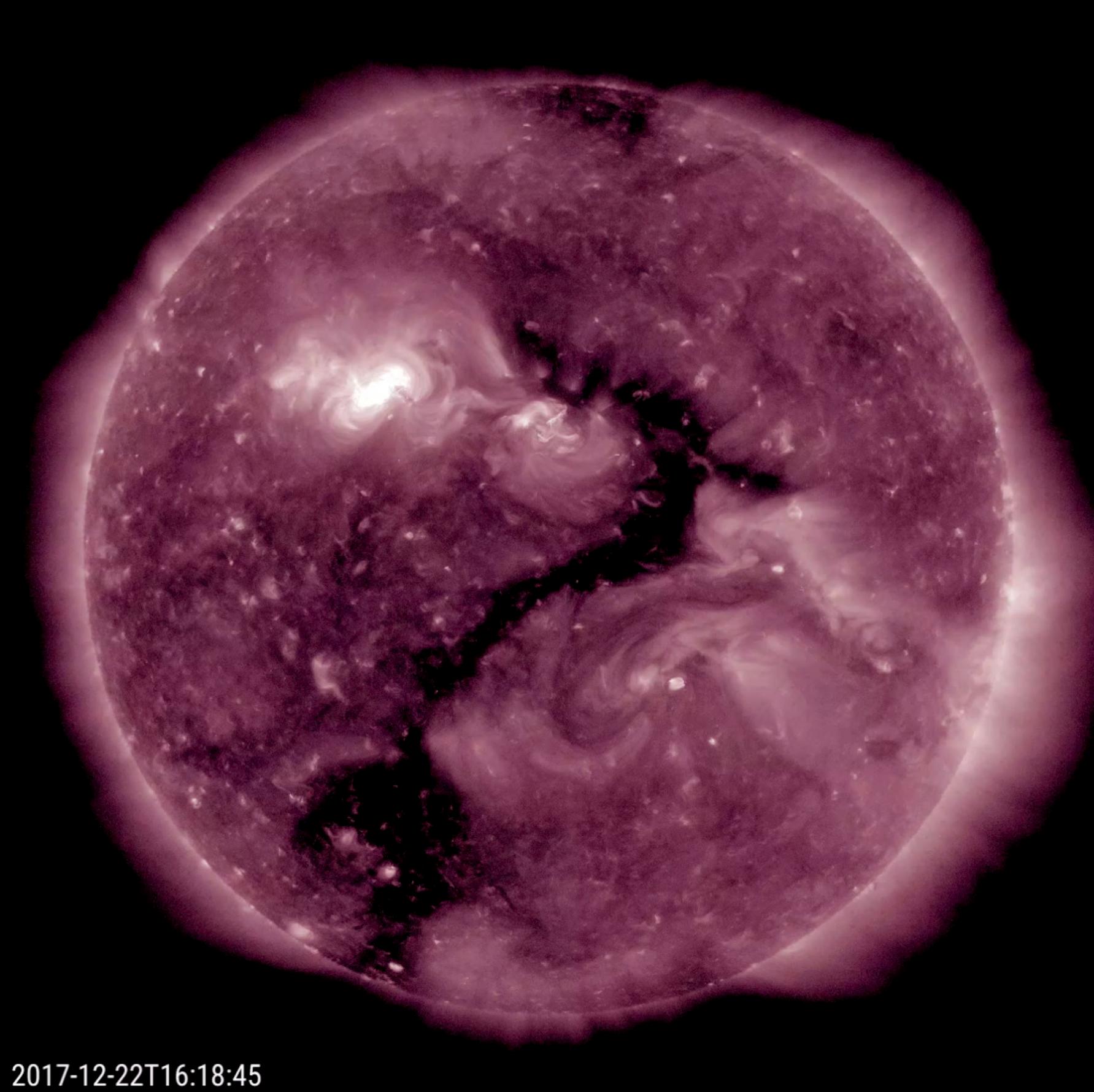
Relative to the third image down on the left: "Oddly enough, an elongated coronal hole (the darker area near the center) seems to shape itself into a single, recognizable question mark over the period of one day (Dec. 21-22, 2017). Coronal holes are areas of open magnetic field that appear darker in extreme ultraviolet light, as is seen here. These holes are the source of streaming plasma that we call solar wind."[60] While the hole is connected to the polar coronal hole it does extend to mid-latitudes.
Mercury[edit | edit source]
.jpg)
.jpg)
"MOST current literature on solar activity assumes that the planets do not affect it, and that conditions internal to the Sun are primarily responsible for the solar cycle. Bigg1, however, has shown that the period of Mercury's orbit appears in the sunspot data, and that the influence of Mercury depends on the phases of Venus, Earth, and Jupiter."[61]
"Some observations show that Mercury is surrounded by a hot corona of calcium atoms with temperature between 12,000 and 20,000 K.[62]"[63]
At right is a diagram of Mercury's sodium tail. "As the MESSENGER spacecraft approached Mercury, the UVVS field of view was scanned across the planet's exospheric "tail," which is produced by the solar wind pushing Mercury's exosphere (the planet's extremely thin atmosphere) outward. This figure, recently published in Science magazine, shows a map of the distribution of sodium atoms as they stream away from the planet (see PIA10396); red and yellow colors represent a higher abundance of sodium than darker shades of blue and purple, as shown in the colored scale bar, which gives the brightness intensity in units of kiloRayleighs. The escaping atoms eventually form a comet-like tail that extends in the direction opposite that of the Sun for many planetary radii. The small squares outlined in black correspond to individual measurements that were used to create the full map. These measurements are the highest-spatial-resolution observations ever made of Mercury's tail. In less than six weeks, on October 6, 2008, similar measurements will be made during MESSENGER's second flyby of Mercury. Comparing the measurements from the two flybys will provide an unprecedented look at how Mercury's dynamic exosphere and tail vary with time."[64]
At left are two diagrams showing the approximate distribution of calcium and magnesium in Mercury's tail. "These figures show observations of calcium and magnesium in Mercury's neutral tail during the third MESSENGER Mercury flyby. The distribution of neutral calcium in the tail appears to be centered near the equatorial plane and the emission rapidly decreases to the north and south as well as in the anti-sunward direction. In contrast, the distribution of magnesium in the tail exhibits several strong peaks in emission and a slower decrease in the north, south, and anti-sunward directions. These distributions are similar to those seen during the second flyby, but the densities were higher during the third flyby, a different "seasonal" variation than for sodium. Studying the changes of the "seasons" for a range of species during MESSENGER's orbital mission phase will be key to quantifying the processes that generate and maintain the exosphere and transport volatile material within the Mercury environment."[65]
Venus[edit | edit source]
"A non-thermal, or “hot”, Venus corona of H atoms has been observed by Mariners 5 and 10 and Venera 9."[66]
"After more than two years in orbit still no Venus Express observations were published concerning the hot oxygen corona of Venus which could verify the corresponding controversial observations of Venera 11 and PVO, three decades ago."[67]
"Venus has a hot oxygen corona in addition to its hydrogen corona (Nagy et al., 1981) and charge-exchange between protons and oxygen is accidentally resonant."[68]
Earth[edit | edit source]

At right is a composite image which contains the first picture of the Earth in X-rays, taken in March, 1996, with the orbiting Polar satellite. The area of brightest X-ray emission is red.
Energetic charged particles from the Sun energize electrons in the Earth's magnetosphere. These electrons move along the Earth's magnetic field and eventually strike the ionosphere, causing the X-ray emission. Lightning strikes or bolts across the sky also emit X-rays.[69]
Mars[edit | edit source]
"Both Earth and Mars have extensive coronae, whereas the Venus corona manifests itself almost entirely within two planetary radii. The Mars corona is relatively thin and exhibits a slight brightening at the dark limb."[70]
Comets[edit | edit source]


"Comet Lulin was passing through the constellation Libra when Swift imaged it on January 28, 2009. The image at right merges data acquired by Swift's Ultraviolet/Optical Telescope (blue and green) and X-Ray Telescope (red). At the time of the observation, the comet was 99.5 million miles from Earth and 115.3 million miles from the Sun."[44]
"NASA's Swift Gamma-ray Explorer satellite was monitoring Comet Lulin as it closed to 63 Gm of Earth. For the first time, astronomers can see simultaneous UV and X-ray images of a comet. "The solar wind -- a fast-moving stream of particles from the sun -- interacts with the comet's broader cloud of atoms. This causes the solar wind to light up with X-rays, and that's what Swift's XRT sees", said Stefan Immler, of the Goddard Space Flight Center. This interaction, called charge exchange, results in X-rays from most comets when they pass within about three times Earth's distance from the sun. Because Lulin is so active, its atomic cloud is especially dense. As a result, the X-ray-emitting region extends far sunward of the comet.[71]"[44]
At left is Comet Lovejoy as detected in STEREO/SECCHI's EUVI-A imager's 17.1-nm wavelength. "The comet is clearly visible racing away from the Sun, leaving a wiggly-tail in its wake! Why the wiggles? We're not sure -- we need to start studying that when we get all of the spacecraft data from STEREO-B this weekend. However, we think there may some kind of helical motion going on, or perhaps there's a projection affect and we're seeing tail material magnetically "clinging" to coronal loops and moving with them. There are other possibilities too, though, and we will certainly investigate those! We should have equivalent images from the STEREO-A spacecraft which we will also get this weekend. When we pair these together, and throw in the SDO images too, we should be able to get an incredibly unique 3-D picture of how this comet is reacting the intense coronal heat and magnetic loops."[72]
Jupiter[edit | edit source]

"Because of an eccentricity of 0.048, the distance from Jupiter and the Sun varies by 75 million km between perihelion and aphelion, or the nearest and most distant points of the planet along the orbital path respectively."[73]
"Favorable oppositions occur when Jupiter is passing through perihelion, an event that occurs once per orbit. As Jupiter approached perihelion in March 2011, there was a favorable opposition in September 2010.[74]"[73]
It's orbital period is 4,332.59 d (11.8618 y).
"It is shown that starting with the alignment of Venus with Jupiter at perihelion position, these two planets will perfectly align at Jupiter's perihelion after every 23.7 years".[75]
"The tidal forces hypothesis for solar cycles has been proposed by Wood (1972) and others. Table 2 below shows the relative tidal forces of the planets on the sun. Jupiter, Venus, Earth and Mercury are called the "tidal planets" because they are the most significant. According to Wood, the especially good alignments of J-V-E with the sun which occur about every 11 years are the cause of the sunspot cycle. He has shown that the sunspot cycle is synchronous with the alignments, and J. Schove's data for 1500 year of sunspot maxima supports the 11.07 year J-V-E period average."[76]
"Both the 11.86 year Jupiter tropical period (time between perihelion's or closest approaches to the sun and the 9.93 year J-S alignment periods are found in sunspot spectral analysis. Unfortunately direct calculations of the tidal forces of all planets does not support the occurrence of the dominant 11.07 year cycle. Instead, the 11.86 year period of Jupiter's perihelion dominates the results. This has caused problems for several researchers in this field."[76]
The "image of Jupiter [at right] shows concentrations of auroral X-rays near the north and south magnetic poles."[77] The Chandra X-ray Observatory accumulated X-ray counts from Jupiter for its entire 10-hour rotation on December 18, 2000.
The coronal cloud around Jupiter is exactly opposite to that around the Sun. At the Sun there are polar coronal holes, whereas at Jupiter the coronal cloud is most prevalent over the magnetic poles.
Saturn[edit | edit source]
"Saturn's corona plays a major role in supplying hydrogen to the circumplanetary volume."[78]
"This cloud probably connects to the extended hydrogen corona of Saturn (Broadfoot et al., 1981; Shemansky and Hall, 1992) and to hydrogen-rich icy surfaces in the inner magnetosphere."[79]
Uranus[edit | edit source]
"The upper part of the thermosphere, where the mean free path of the molecules exceeds the scale height, [The scale height sh is defined as sh = RT/(Mgj), where R = 8.31 J/mol/K is the gas constant, M ≈ 0.0023 kg/mol is the average molar mass in the Uranian atmosphere,[80] T is temperature and gj ≈ 8.9 m/s2 is the gravitational acceleration at the surface of Uranus. As the temperature varies from 53 K in the tropopause up to 800 K in the thermosphere, the scale height changes from 20 to 400 km.] is called the exosphere.[81] The lower boundary of the Uranian exosphere, the exobase, is located at a height of about 6,500 km, or 1/4 of the planetary radius, above the surface.[81] The exosphere is unusually extended, reaching as far as several Uranian radii from the planet.[81][82] It is made mainly of hydrogen atoms and is often called the hydrogen corona of Uranus.[83] The high temperature and relatively high pressure at the base of the thermosphere explain in part why Uranus's exosphere is so vast. The corona contains a significant population of supra-thermal (energy of up to 2 eV) hydrogen atoms. Their origin is unclear, but they may be produced by the same mechanism that heats the thermosphere.[81][82] The number density of atomic hydrogen in the corona falls slowly with the distance from the planet, remaining as high a few hundred atoms per cm3 at a few radii from Uranus.[81] The effects of this bloated exosphere include a drag on small particles orbiting Uranus, causing a general depletion of dust in the Uranian rings. The infalling dust in turn contaminates the upper atmosphere of the planet.[83]"[84]
Epsilon Eridani[edit | edit source]
"Epsilon Eridani has a higher level of magnetic activity than the Sun, and hence demonstrates increased activity in the outer parts of the star's atmosphere: the chromosphere and corona. The average magnetic field strength of this star across the entire surface is (1.65 ± 0.30) × 10−2 T,[85] which is more than forty times greater than the (5–40) × 10−5 T magnetic field strength in the Sun's photosphere.[86]"[87]
"The X-ray luminosity of Epsilon Eridani is about 2 × 1028 ergs/s (2 × 10²¹ W). It is brighter in X-ray emission than the Sun at peak activity. The source for this strong X-ray emission is the star's hot corona.[88][89] Epsilon Eridani's corona appears larger and hotter than the Sun's, with a temperature of 3.4 × 10⁶ K as measured from observation of the corona's ultraviolet and X-ray emission.[90]"[87]
"The stellar wind emitted by Epsilon Eridani expands until it collides with the surrounding interstellar medium of sparse gas and dust, resulting in a bubble of heated hydrogen gas. The absorption spectrum from this gas has been measured with the Hubble Space Telescope, allowing the properties of the stellar wind to be estimated.[90] Epsilon Eridani's hot corona results in a mass loss rate from the star's stellar wind that is 30 times higher than the Sun's. This wind is generating an astrosphere (the equivalent of the heliosphere that surrounds the Sun) that spans about 8,000 AU and contains a bow shock that lies 1,600 AU from the star. At its estimated distance from Earth, this astrosphere spans 42 arcminutes, which is wider than the apparent size of the full Moon.[91]"[87]
Gliese 176[edit | edit source]
"The corona of this star has a moderate emission of X-rays at 3 × 1027 erg s–1. This indicates the star is active, and may exhibit starspots and flares much like the Sun. This is considered normal for a main-sequence star of spectral class M."[92]
Local hot bubbles[edit | edit source]

The 'local hot bubble' is a "hot X-ray emitting plasma within the local environment of the Sun."[93] "This coronal gas fills the irregularly shaped local void of matter (McCammon & Sanders 1990) - frequently called the Local Hot Bubble (LHB)."[93]
Def. a "hot X-ray emitting plasma within the local environment of the Sun"[93] is called the Local Hot Bubble.
"The [X-ray] intensity of the [Local Hot Bubble] LHB varies across the entire sky:"[94]
- ILHB = (2.5-8.2) x 10-4 cts s-1 arcmin-2 (Snowden et al. 1998).
The galactic X-ray background is produced largely by emission from the Local Hot Bubble which is within 100 parsecs of the Sun. The Local Hot Bubble is within the Local Bubble.
White dwarfs[edit | edit source]
"The white dwarf is surrounded by an expanding shell of gas in an object known as a planetary nebula. Planetary nebulae seem to mark the transition of a medium mass star from red giant to white dwarf. X-ray images reveal clouds of multimillion degree gas that have been compressed and heated by the fast stellar wind."[44]
Chamaeleon I dark clouds[edit | edit source]

"The Chamaeleon I (Cha I) cloud is a coronal cloud and one of the nearest active star-forming regions at ~160 pc.[95] It is relatively isolated from other star-forming clouds, so it is unlikely that older pre-main sequence (PMS) stars have drifted into the field.[95] The total stellar population is 200-300.[95] The Cha I cloud is further divided into the North cloud or region and South cloud or main cloud."[44]
Chamaeleon II dark clouds[edit | edit source]
"The Chamaeleon II dark cloud contains some 40 X-ray sources.[96] Observation in Chamaeleon II was carried out from September 10 to 17, 1993.[96] Source RXJ 1301.9-7706, a new WTTS candidate of spectral type K1, is closest to 4U 1302-77.[96]"[44]
Chamaeleon III dark clouds[edit | edit source]
"Chamaeleon III appears to be devoid of current star-formation activity."[97] "HD 104237 (spectral type A4e) observed by [the Advanced Satellite for Cosmology and Astrophysics (ASCA)], located in the Chamaeleon III dark cloud, is the brightest Herbig Ae/Be star in the sky.[98]"[44]
Galactic coronal clouds[edit | edit source]
"Discussion of the alternative hypothesis of cloud ejection from the equatorial layer of the Galaxy leads to the conclusion that the gaseous halo must be highly turbulent and that the coronal clouds are probably H I regions".[99]
"One question posed by these previous observations is where the absorption originates. If a coronal cloud, the cloud is more than 15 kpc from the plane of NGC 3067. This distance is greater than the optical radius of the galaxy, 9.6 kpc (H = 50 km s-1 Mpc-1. Furthermore, the narrow line requires that the cloud be cool, in contrast to the wide range of ionization stages detected for the corona of our Galaxy (Savage and deBoer 1981)."[100] "But if the cloud originates instead in the disk, and is moving in a circular orbit viewed at an inclination of 68 deg (the inclination of the optical galaxy), then some gas extends at least to 40 kpc, which is over four times the optical radius."[100]
Quasars[edit | edit source]
Def. "[a]n extragalactic object, starlike in appearance, that is among the most luminous ... objects in the universe"[101] is called a quasar.
3C 273 is a quasar located in the constellation Virgo. "In the 3C 273 case the emitting area would be about 3000 AU across if the emission were Planckian at 17,000 K, but this could be spread out over many smaller clouds, as suggested by Krolik and McKee."[54]
Interacting galaxies[edit | edit source]
In the image at right of The Antennae, the top image, a wide field X-ray view, reveals spectacular loops of hot gas spreading out from the southern part of The Antenna into intergalactic space. In the closeup view on the lower left, the point sources have been taken out to emphasize the hot gas clouds in the central regions of The Antennae. The image at the lower right is processed and color-coded to show regions rich in iron (red), magnesium (green) and silicon (blue).
"From the Chandra X-ray analysis of the Antennae Galaxies rich deposits of neon, magnesium, and silicon were discovered. These elements are among those that form the building blocks for habitable planets. The clouds imaged contain magnesium and silicon at 16 and 24 times respectively, the abundance in the Sun."[44]
Galaxy clusters[edit | edit source]


3C 295 is a strongly X-ray emitting galaxy cluster in the constellation Boötes. 3C 295 (Cl 1409+524) "is one of the most distant galaxy clusters observed by X-ray telescopes. The cluster is filled with a vast cloud of 50 MK gas that radiates strongly in X rays. [The Chandra X-ray Observatory detected] that the central galaxy is a strong, complex source of X rays."[44] The cluster is located at J 2000.0 RA 14h 11m 20s Dec −52° 12' 21". Observation date for the Chandra image is August 30, 1999.
The Perseus galaxy cluster is located at J 2000.0 RA 03h 19m 47.60s Dec +41° 30' 37.00". The observation dates for the image at right of 13 pointings are between August 8, 2002, and October 20, 2004. "The Perseus galaxy cluster is one of the most massive objects in the universe, containing thousands of galaxies immersed in a vast cloud of multimillion degree gas."[44]
Databases[edit | edit source]
From the SIMBAD data base is a collection of objects which are both astronomical X-ray sources and coronal clouds.
| Source | Abbreviation | Number | Known X-ray sources | Known gamma-ray sources (gam) |
|---|---|---|---|---|
| Active galactic nucleus | AGN | 34,232 | 6265 | 386 |
| Astronomical gamma-ray source | gam + gB | 1872 + 7638 | 986 + 23 | 1872 |
| Astronomical infrared source | IR | 1,888,729 | 28,497 | 484 |
| Astronomical blue source | blu | 19,323 | 383 | 31 |
| Astronomical radio source | Rad | 487,066 | 5211 | 409 |
| Astronomical red source | red | 269 | 17 | 0 |
| Astronomical ultraviolet source | UV | 87,216 | 2767 | 119 |
| Astronomical X-ray source | X | 203,637 | 203,637 | 986 |
| Cloud | Cld | 8379 | 4 | 0 |
| Dark nebula | DNe | 20,972 | 6 | 1 |
| Dwarf nova | DN* | 478 | 82 | 2 |
| Emission object | EmO | 11,837 | 181 | 9 |
| Galaxy | G | 1,287,663 | 5984 | 397 |
| HI region | HI | 5724 | 36 | 7 |
| HII region | HII | 25,654 | 198 | 6 |
| Interstellar medium | ISM | 4530 | 66 | 1 |
| Molecular cloud | MoC | 5679 | 7 | 3 |
| Nova | No* | 1360 | 74 | 13 |
| Nova-like star | NL* | 103 | 27 | 0 |
| Open galactic cluster | OpC | 2161 | 21 | 0 |
| Planetary nebula | PN | 10,737 | 48 | 2 |
| Quasar | QSO | 148,801 | 5796 | 323 |
| Reflection nebula | RNe | 1799 | 7 | 0 |
| Star | * | 1,792,160 | 18,291 | 227 |
| Supernova | SN | 6391 | 21 | 7 |
| Supernova remnant | SNR | 1166 | 246 | 29 |
| Young stellar object | Y*O | 8151 | 1694 | 0 |
Locations on Earth[edit | edit source]
"Global maps illustrate the geographic region of visibility for each eclipse."[102]
Recent history[edit | edit source]
The recent history period dates from around 1,000 b2k to present. Initially the concept of a coronal cloud developed with observations of clouds or cloud-like structures forming above the photospheric surface of the Sun.
"Coronal clouds, type IIIg, form in space above a spot area and rain streamers upon it."[103] Type IIIg is a subdivision of sunspot prominences (class III).[103] "Occasionally dots form in space above a sunspot group. Other dots then appear, and all coalesce into a suspended cloud from which streamers pour into the spot area."[103]
"Occasionally one member of an interactive group has been a tornado prominence, but, for the first time, on January 4, 1945, a coronal cloud prominence of the sunspot class was observed to participate in such an interaction."[104] "The coronal cloud prominence ... formed in space, and from it streamers flowed into a neighboring prominence instead of into a spot area on the sun as is usual with coronal prominences."[104] "On January 5, a surge was photographed over the spot area, the coronal cloud being still visible. On January 6, a trace of the cloud was visible, but solar rotation soon carried the whole interactive group from the limb. The coronal cloud probably endured at least 2 days."[104]
"On December 18, 1956, a large and active sunspot region was at the west limb of the sun."[105] "Continuous emission from a dense coronal cloud was observed just before the flare. This cloud condenses sharply during the flare and dissipates afterward."[105] After a second class 2 flare occurred at 2131 U.T., "[a]t about 2200 U.T. a bright cloud appeared above the limb at the active region, reaching maximum surface brightness at 2208 and maximum total brightness at around 2220."[105] "The flare at 2200 (the bright cloud) appears larger and brighter on the coronagraph photographs, but we are definitely looking at the same object."[105] The initial "flare appears to have been a violent condensation of material from a dense coronal cloud above an active region."[105] "The coronal temperature was 4000000°."[105]
Energies[edit | edit source]
"[I]t appears that the energy requirements of coronal hole regions of the solar surface are substantially greater than those of other regions. The main factor determining this conclusion is an estimate of the energy required to accelerate the solar wind in regions above coronal holes. ... Alfven waves [are] more easily accommodated [by the energy budget than thermal plasma pressure]."[106]
Magnetohydrodynamics[edit | edit source]
Def. "the study of the interaction of electrically conducting fluids with magnetic fields"[107] is called magnetohydrodynamics (MHD).
In a coronal cloud are magnetohydrodynamic plasma flux tubes along magnetic field lines.[20]
"[M]otions resulting from [a linear magnetohydrodynamic] instability act as a dynamo to sustain the magnetic field."[108] "Supersonic flows are initially generated by the Balbus-Hawley magnetic shear instability."[108] "A plasma with local magnetohydrodynamic instabilities creates mechanical turbulence, motion, or shear (a dynamo) which in turn generates or sustains the local magnetic field."[109]
Catalogs[edit | edit source]
"This catalog contains all the CMEs [about 7000] detected by the LASCO coronagraphs C2 and C3, which cover a combined field of view of 2.1 to 32 Rs."[110]
Technology[edit | edit source]


One of the objectives of the Stardust mission, specifically the Dynamic Science Experiment (DSE), is to "[s]ound the solar corona at X band [ radio astronomy ], including electron content of the inner corona, solar wind acceleration, turbulence, and a search for coronal mass ejections."[111]
"Suisei [at left] began UV observations in Nov. 1985, generating up to 6 images/day. The spacecraft encountered Comet P/Halley at 151,000 km on sunward side during March 8, 1986, suffering only 2 dust impacts."[112]
"Suisei took a lot of UV pictures of the neutral hydrogen corona around the comet [Comet P/Halley]".[113]
Hypotheses[edit | edit source]
- The volume of plasma objects is greater than the volume of cold regions.
See also[edit | edit source]
References[edit | edit source]
- ↑ 1.0 1.1 R. P. Lin; H. S. Hudson (September-October 1976). "Non-thermal processes in large solar flares". Solar Physics 50 (10): 153-78. doi:10.1007/BF00206199. http://adsabs.harvard.edu/full/1976SoPh...50..153L. Retrieved 2013-07-07.
- ↑ A. Bhardwaj; R. Elsner (February 20, 2009). "Earth Aurora: Chandra Looks Back At Earth". Cambridge, Massachusetts, USA: Harvard-Smithsonian Center for Astrophysics. Retrieved 2013-05-10.
- ↑ Ulmshneider, Peter (1997). Heating of Chromospheres and Coronae in Space Solar Physics, Proceedings, Orsay, France, edited by J.C. Vial, K. Bocchialini and P. Boumier. Springer. pp. 77–106. ISBN 3-540-64307-9.
- ↑ Malara F., Velli M. (2001). Observations and Models of Coronal Heating in Recent Insights into the Physics of the Sun and Heliosphere: Highlights from SOHO and Other Space Missions, Proceedings of IAU Symposium 203, edited by Pål Brekke, Bernhard Fleck, and Joseph B. Gurman. Astronomical Society of the Pacific. pp. 456–466. ISBN 1-58381-069-2.
- ↑ corona. San Francisco, California: Wikimedia Foundation, Inc. May 9, 2012. http://en.wiktionary.org/wiki/corona. Retrieved 2012-06-28.
- ↑ S. Patsourakos; J.-C. Vial (2002). "Intermittent behavior in the transition region and the low corona of the quiet Sun". Astronomy and Astrophysics 385: 1073–1077. doi:10.1051/0004-6361:20020151.
- ↑ Steve Cole; Jia-Rui C. Cook; Alan Buis (December 2011). "NASA's Voyager Hits New Region at Solar System Edge". Washington, DC: NASA. Retrieved 2012-02-09.
- ↑ Kent S. Wood; Peter F. Michelson; Mallory S. Roberts (1996). "A Modified Beat Frequency Modulated Accretion Model I. Spin Periods and Magnetic Moments of Z-Sources Inferred from Horizontal Branch QPO". Palo Alto, California USA: Stanford University. Retrieved 2013-07-10.
- ↑ E. Tandberg-Hanssen (1977). A. Bruzek and C. J. Durrant. ed. Prominences, In: Illustrated Glossary for Solar and Solar-Terrestrial Physics. Dordrecht-Holland: D. Reidel Publishing Company. pp. 97-109. doi:10.1007/978-94-010-1245-4_10. ISBN 978-94-010-1247-8. http://link.springer.com/chapter/10.1007/978-94-010-1245-4_10. Retrieved 2013-07-10.
- ↑ 10.0 10.1 Leon Golub; Harold Zirin; Haimin Wang (August 1994). "The roots of coronal structure in the Sun's surface". Solar Physics 153 (1-2): 179-98. doi:10.1007/BF00712500. http://link.springer.com/article/10.1007/BF00712500. Retrieved 2013-07-10.
- ↑ 11.0 11.1 11.2 Martin Koomen; Russell Howard; Richard Hansen; Shirley Hansen (February 1974). "The coronal transient of 16 June 1972". Solar Physics 34 (2): 447-52. doi:10.1007/BF00153680. http://link.springer.com/article/10.1007/BF00153680. Retrieved 2013-07-10.
- ↑ 12.0 12.1 Katsuo Tanaka, Harold Zirin (December 15, 1985). "The great flare of 1982 June 6". The Astrophysical Journal 299 (12): 1036-46. doi:10.1086/163771. http://adsabs.harvard.edu/full/1985ApJ...299.1036T. Retrieved 2013-07-10.
- ↑ Hugh S. Hudson; D. F. Webb (1997). N. Crooker. ed. Soft X-ray signatures of coronal ejections, In: Coronal Mass Ejections. Geophysical Monograph Series. 99. Washington, DC USA: American Geophysical Union. pp. 27-38. doi:10.1029/GM099p0027. http://www.agu.org/books/gm/v099/GM099p0027/GM099p0027.shtml. Retrieved 2013-07-10.
- ↑ H. Zirin; U. Feldman; G. A. Doschek; S. Kane (May 15, 1981). "On the relationship between soft X-rays and Hα-emitting structures during a solar flare". The Astrophysical Journal 246 (05): 321-30. doi:10.1086/158925. http://adsabs.harvard.edu/full/1981ApJ...246..321Z. Retrieved 2013-07-10.
- ↑ S. Masuda; T. Kosugi; Hugh S. Hudson (December 2001). "A hard X-ray two-ribbon flare observed with Yohkoh/HXT". Solar Physics 204 (1-2): 57-69. doi:10.1023/A:1014230629731. http://link.springer.com/article/10.1023/A:1014230629731. Retrieved 2013-07-10.
- ↑ Hugh S. Hudson (1997). N. Crooker. ed. Solar antecedents of geomagnetic storms, In: Coronal Mass Ejections. Geophysical Monograph Series. 99. Washington, DC USA: American Geophysical Union. pp. 27-38. doi:10.1029/GM099p0027. http://www.agu.org/books/gm/v099/GM099p0027/GM099p0027.shtml. Retrieved 2013-07-10.
- ↑ James F. Steiner; Rubens C. Reis; Andrew C. Fabian; Ronald A. Remillard; Jeffrey E. McClintock; Lijun Gou; Ryan Cooke; Laura W. Brenneman et al. (December 11, 2012). "A broad iron line in LMC X‐1". Monthly Notices of the Royal Astronomical Society 427 (3): 2552-61. doi:10.1111/j.1365-2966.2012.22128.x. http://onlinelibrary.wiley.com/doi/10.1111/j.1365-2966.2012.22128.x/full. Retrieved 2013-07-10.
- ↑ R. Tousey (July 16, 1971). "Chromosphere and Corona: Observations of the Extreme Ultraviolet Solar Spectrum". Philosophical Transactions of the Royal Society London. A Mathematical, Physical & Engineering Sciences 270 (1202): 59-70. doi:10.1098/rsta.1971.0060. http://rsta.royalsocietypublishing.org/content/270/1202/59.short. Retrieved 2013-07-10.
- ↑ H. Zirin (May 1997). "Is There a Background Polar Field?". Bulletin of the American Astronomical Society 29 (05): 902. http://esoads.eso.org/abs/1997SPD....28.0250Z. Retrieved 2013-07-10.
- ↑ 20.0 20.1 Markus J. Aschwanden (2007). Erdelyi R. ed. "Fundamental Physical Processes in Coronae: Waves, Turbulence, Reconnection, and Particle Acceleration In: Waves & Oscillations in the Solar Atmosphere: Heating and Magneto-Seismology". Proceedings IAU Symposium 3 (S247): 257–68. doi:10.1017/S1743921308014956. http://journals.cambridge.org/download.php?file=%2FIAU%2FIAU3_S247%2FS1743921308014956a.pdf&code=7c95b408db74ccbe9f1f376d4cb1ef35.
- ↑ Massey P; Silva DR; Levesque EM; Plez B; Olsen KAG; Clayton GC; Meynet G; Maeder A (2009). "Red Supergiants in the Andromeda Galaxy (M31)". The Astrophysical Journal 703 (1): 420. doi:10.1088/0004-637X/703/1/420.
- ↑ 22.0 22.1 22.2 22.3 22.4 Erdèlyi R; Ballai I (2007). "Heating of the solar and stellar coronae: a review". Astron Nachr 328 (8): 726. doi:10.1002/asna.200710803.
- ↑ Russell CT (2001). "Solar wind and interplanetary magnetic field: A tutorial". In Song, Paul. Space Weather (Geophysical Monograph). American Geophysical Union. pp. 73–88. ISBN 9780875909844. http://www-ssc.igpp.ucla.edu/personnel/russell/papers/SolWindTutorial.pdf.
- ↑ Alfvén H (1947). "Magneto-hydrodynamic waves, and the heating of the solar corona". Monthly Notices of the Royal Astronomical Society 107: 211.
- ↑ Parker EN (1988). "Nanoflares and the solar X-ray corona". The Astrophysical Journal 330: 474. doi:10.1086/166485.
- ↑ Sturrock PA, Uchida Y (1981). "Coronal heating by stochastic magnetic pumping". The Astrophysical Journal 246: 331. doi:10.1086/158926.
- ↑ "X-ray astronomy, In: Wikipedia". San Francisco, California: Wikimedia Foundation, Inc. June 11, 2012. Retrieved 2012-06-29.
- ↑ Burlaga, L. F., E. Sittler, F. Mariani, and R. Schwenn, "Magnetic loop behind an interplanetary shock: Voyager, Helios and IMP-8 observations" in "Journal of Geophysical Research", 86, 6673, 1981
- ↑ Burlaga, L. F. et al., "A magnetic cloud and a coronal mass ejection" in "Geophysical Research Letter"s, 9, 1317-1320, 1982
- ↑ Lepping, R. P. et al. "Magnetic field structure of interplanetary magnetic clouds at 1 AU" in "Journal of Geophysical Research", 95, 11957-11965, 1990.
- ↑ coronal mass ejection. San Francisco, California: Wikimedia Foundation, Inc. June 21, 2013. http://en.wiktionary.org/wiki/coronal_mass_ejection. Retrieved 2013-07-07.
- ↑ 32.0 32.1 32.2 32.3 32.4 Harold Zirin (October 1964). "The Limb Flare of November 20, 1960: a Coronal Phenomenon". Astrophysical Journal 140 (10): 1216-35. doi:10.1086/148019.
- ↑ 33.0 33.1 33.2 Gopalswamy N; Mikic Z; Maia D; Alexander D; Cremades H; Kaufmann P; Tripathi D; Wang YM (2006). "The pre-CME Sun". Space Sci Rev 123 (1–3): 303. doi:10.1007/s11214-006-9020-2.
- ↑ K. H. Schatten, D. J. Mullan (December 1, 1977). "Fast azimuthal transport of solar cosmic rays via a coronal magnetic bottle". Journal of Geophysical Research 82 (35): 5609-20. doi:10.1029/JA082i035p05609. http://www.agu.org/pubs/crossref/1977/JA082i035p05609.shtml. Retrieved 2013-07-07.
- ↑ H. Zinn (1965). C. C. Chang and S. S. Huang. ed. Solar Flares and Concurrent Phenomena in the Solar Atmosphere, In: Proceedings of the Plasma Space Science Symposium. 3. Netherlands: Springer. pp. 38-51. doi:10.1007/978-94-011-7542-5_5. ISBN 978-94-011-7544-9. http://link.springer.com/chapter/10.1007/978-94-011-7542-5_5. Retrieved 2013-07-07.
- ↑ A. Markowitz; R. Edelson (December 20, 2004). "An expanded Rossi X-ray timing explorer survey of X-ray variability in Seyfert 1 galaxies". The Astrophysical Journal 617 (2): 939-65. doi:10.1086/425559. http://iopscience.iop.org/0004-637X/617/2/939. Retrieved 2013-07-07.
- ↑ A. Bellerive, Review of solar neutrino experiments. Int.J.Mod.Phys. A19 (2004) 1167-1179
- ↑ "Solar neutrino, In: Wikipedia". San Francisco, California: Wikimedia Foundation, Inc. April 4, 2012. Retrieved 2012-11-08.
- ↑ K.D. Abhyankar (1977). "A Survey of the Solar Atmospheric Models". Bull. Astr. Soc. India 5: 40–44. http://prints.iiap.res.in/handle/2248/510.
- ↑ "Sun, In: Wikipedia". San Francisco, California: Wikimedia Foundation, Inc. June 29, 2013. Retrieved 2013-07-07.
- ↑ 41.0 41.1 J. N. Bahcall; G. B. Field; W. H. Press (September 1, 1987). "Is solar neutrino capture rate correlated with sunspot number?". The Astrophysical Journal 320 (9): L69-73. doi:10.1086/184978. http://articles.adsabs.harvard.edu//full/1987ApJ...320L..69B/L000069.000.html. Retrieved 2013-07-07.
- ↑ 42.0 42.1 42.2 O. V. Terekhov; R. A. Syunyaev; A. V. Kuznetsov; C. Barat; R. Talon; G. Trottet; N. Vilmer (March 1993). "Deuterium synthesis in the solar flare on 24 May 1990: observations of delayed emission in the 2.2 Mev γ-ray line by the GRANAT satellite". Astronomy Letters 19 (03): 65-8.
- ↑ 43.0 43.1 Maurice Dubin; Robert K. Soberman (April 1996). "Resolution of the Solar Neutrino Anomaly". arXiv: 1-8. http://arxiv.org/abs/astro-ph/9604074. Retrieved 2012-11-11.
- ↑ 44.00 44.01 44.02 44.03 44.04 44.05 44.06 44.07 44.08 44.09 "Astrophysical X-ray source, In: Wikipedia". San Francisco, California: Wikimedia Foundation, Inc. June 12, 2012. Retrieved 2012-06-28.
- ↑ 45.0 45.1 Holly Zell (August 4, 2010). Spacecraft Observes Coronal Mass Ejection. Washington, DC USA: NASA. http://www.nasa.gov/topics/solarsystem/sunearthsystem/main/News080210-cme.html. Retrieved 2013-07-07.
- ↑ Robert Nemiroff; Jerry Bonnell (August 28, 1999). X-Ray Pleiades. Greenbelt, Maryland USA: NASA/GSFC. http://apod.nasa.gov/apod/ap990828.html. Retrieved 2013-07-07.
- ↑ Lynn Jenner (November 30, 2007). "NASA Shares Solar Eclipse With the World". Washington, DC USA: NASA. Retrieved 2013-07-08.
- ↑ 48.0 48.1 48.2 P. Swings (July 1943). "Edlén's Identification of the Coronal Lines with Forbidden Lines of Fe X, XI, XIII, XIV, XV; Ni XII, XIII, XV, XVI; Ca XII, XIII, XV; a X, XIV". The Astrophysical Journal 98 (07): 116-28. doi:10.1086/144550.
- ↑ 49.0 49.1 49.2 M. Minnaert (1930). "On the continuous spectrum of the corona and its polarisation". Zeitschrift für Astrophysik 1: 209-36. http://adsabs.harvard.edu/abs/1930ZA......1..209M. Retrieved 2013-07-08.
- ↑ Wang, Y. M., et al., Multiple magnetic clouds in interplanetary space, Solar Physics, 211, 333-344, 2002.
- ↑ Wang, Y. M., et al., Multiple magnetic clouds: Several examples during March - April, 2001, J. Geophys. Res., 108(A10), 1370, 2003.
- ↑ "Magnetic cloud, In: Wikipedia". San Francisco, California: Wikimedia Foundation, Inc. December 5, 2012. Retrieved 2013-07-07.
- ↑ 53.0 53.1 Jan Olof Stenflo (15 July 2004). "Solar physics: Hidden magnetism". Nature 430 (6997): 304-5. doi:10.1038/430304a. http://www.nature.com/nature/journal/v430/n6997/full/430304a.html. Retrieved 2015-09-21.
- ↑ 54.0 54.1 54.2 54.3 Harold Zirin (June 1978). "The L-alpha/H-alpha ratio in solar flares, quasars, and the chromosphere". Astrophysical Journal 222 (6): L105-7. doi:10.1086/182702.
- ↑ 55.0 55.1 55.2 55.3 McWhirter, R. W. P.; Kopp, R. A. (September 1979). "The energy balance in the solar atmosphere above coronal holes". Royal Astronomical Society, Monthly Notices 188 (9): 871-81.
- ↑ 56.0 56.1 R. Schwenn; B. Inhester; S. P. Plunkett; A. Epple; B. Podlipnik; D. K. Bedford; C. J. Eyles; G. M. Simnett et al. (October 1997). "First View of the Extended Green-Line Emission Corona At Solar Activity Minimum Using the Lasco-C1 Coronagraph on Soho". Solar Physics 175 (2): 667-84. doi:10.1023/A:1004948913883. http://www.springerlink.com/index/R10HN0R60R081237.pdf. Retrieved 2012-02-17.
- ↑ 57.0 57.1 57.2 57.3 Megan Garber (5 June 2013). No Big Deal, Just a Giant Hole in the Sun. The Atlantic. http://www.theatlantic.com/technology/archive/2013/06/no-big-deal-just-a-giant-hole-in-the-sun/276564/. Retrieved 2015-05-18.
- ↑ NASA/Goddard/SDO (17 March 2015). Two Coronal Holes on the Sun Viewed by SDO. Greenbelt, Maryland USA: Goddard Space Flight Center. pp. 1. https://www.flickr.com/people/24662369@N07. Retrieved 2018-02-07.
- ↑ NASA/SDO (15 October 2015). Coronal Hole Front and Center. Greenbelt, Maryland USA: GSFC. pp. 1. https://www.nasa.gov/image-feature/goddard/coronal-hole-front-and-center. Retrieved 2018-02-07.
- ↑ NASA/GSFC/Solar Dynamics Observatory (29 December 2017). PIA22197: The Sun Forms a Question. Greenbelt, Maryland USA: GSFC. pp. 1. https://photojournal.jpl.nasa.gov/jpeg/PIA22197.jpg. Retrieved 2018-02-07.
- ↑ K. D. Wood (November 10, 1972). "Physical Sciences: Sunspots and Planets". Nature 240 (5376): 91-3. doi:10.1038/240091a0. http://www.nature.com/nature/journal/v240/n5376/abs/240091a0.html. Retrieved 2013-07-07.
- ↑ Rosemary Killen; Gabrielle Cremonese; Helmut Lammer (2007). "Processes that Promote and Deplete the Exosphere of Mercury". Space Science Reviews 132 (2-4): 433–509. doi:10.1007/s11214-007-9232-0.
- ↑ "Atmosphere of Mercury, In: Wikipedia". San Francisco, California: Wikimedia Foundation, Inc. May 29, 2013. Retrieved 2013-07-09.
- ↑ Sue Lavoie (August 26, 2008). "PIA11076: Exploring Mercury's "Tail"". Pasadena, California USA: NASA/JPL. Retrieved 2013-07-09.
- ↑ Sue Lavoie (November 5, 2009). "PIA12366: Calcium and Magnesium in Mercury's Exosphere". Pasadena, California USA: NASA/JPL. Retrieved 2013-07-09.
- ↑ S. Kumar; D.M. Hunten; A.L. Broadfoot (November 1978). "Non-thermal hydrogen in the Venus exosphere: The ionospheric source and the hydrogen budget". Planetary and Space Science 26 (11): 1063-75. doi:10.1016/0032-0633(78)90029-6. http://www.sciencedirect.com/science/article/pii/0032063378900296. Retrieved 2013-07-10.
- ↑ H. I. M. Lichtenegger; H. Gröller; H Lammer; Yu. N. Kulikov; V. I. Shematovich (May 2009). "On the elusive hot oxygen corona of Venus". Geophysical Research Letters 36 (10). doi:10.1029/2009GL037575. http://onlinelibrary.wiley.com/doi/10.1029/2009GL037575/full. Retrieved 2013-07-10.
- ↑ C. T. Russell; T. I. Gombosi; M. Horanyi; T. E. Cravens; A. F. Nagy (February 1983). "Charge‐exchange in the magnetosheaths of Venus and Mars: A comparison". Geophysical Research Letters 10 (2): 163-4. doi:10.1029/GL010i002p00163. http://onlinelibrary.wiley.com/doi/10.1029/GL010i002p00163/full. Retrieved 2013-07-10.
- ↑ Newitz, A. (2007) Educated Destruction 101. Popular Science magazine, September. pg. 61.
- ↑ Donald E. Anderson Jr., Charles W. Hord (June 1977). "Multidimensional radiative transfer: Applications to planetary coronae". Planetary and Space Science 25 (6): 563-71. doi:10.1016/0032-0633(77)90063-0. http://www.sciencedirect.com/science/article/pii/0032063377900630. Retrieved 2013-07-10.
- ↑ F Reddy. "NASA's Swift Spies Comet Lulin".
- ↑ Karl Battams (December 2, 2011). "The Great "Birthday Comet" of 2011, Chapter 2: Survival". Washington, DC, USA: Naval Research Laboratory. Retrieved 2013-07-07.
- ↑ 73.0 73.1 "Jupiter, In: Wikipedia". San Francisco, California: Wikimedia Foundation, Inc. July 5, 2013. Retrieved 2013-07-07.
- ↑ Horizons output. "Favorable Appearances by Jupiter". Retrieved 2008-01-02. (Horizons)
- ↑ S.D. Verma (1986). K. B. Bhatnagar. ed. Influence of Planetary Motion and Radial Alignment of Planets on Sun, In: Space Dynamics and Celestial Mechanics. 127. Springer Netherlands. pp. 143-54. doi:10.1007/978-94-009-4732-0_13. ISBN 978-94-010-8603-5. http://link.springer.com/chapter/10.1007/978-94-009-4732-0_13. Retrieved 2013-07-07.
- ↑ 76.0 76.1 Ray Tomes (February 1990). Towards a Unified Theory of Cycles. Cycles Research Institute. pp. 21. http://cyclesresearchinstitute.org/cycles-general/tomes_unified_cycles.pdf. Retrieved 2013-07-07.
- ↑ NASA/CXC/SWRI/G.R.Gladstone (February 27, 2002). "Jupiter Hot Spot Makes Trouble For Theory". Cambridge, Massachusetts: Harvard-Smithsonian Center for Astrophysics. Retrieved 2012-07-11.
- ↑ W.H. Smyth, M.R. Combi (November 1, 1987). "Extended atmospheres of outer planet satellites and comets. Interim report, 15 June-14 September 1987". p. 122. Retrieved 2013-07-10.
- ↑ D. T. Young; J. J. Berthelier; M. Blanc; J. L. Burch; A. J. Coates; R. Goldstein; M. Grande; T. W. Hill et al. (September 2004). "Cassini plasma spectrometer investigation". Space Science Reviews 114 (1-4): 1-112. doi:10.1007/s11214-004-1406-4. http://link.springer.com/article/10.1007/s11214-004-1406-4. Retrieved 2013-07-10.
- ↑ Lunine, Jonathan I. (September 1993). "The Atmospheres of Uranus and Neptune". Annual Review of Astronomy and Astrophysics 31: 217–263. doi:10.1146/annurev.aa.31.090193.001245.
- ↑ 81.0 81.1 81.2 81.3 81.4 Herbert, Floyd; Hall, Doyle T. (May 1996). "Atomic hydrogen corona of Uranus". Journal of Geophysical Research 101 (A5): 10,877–10,885. doi:10.1029/96JA00427.
- ↑ 82.0 82.1 Herbert, Floyd; Sandel, Bill R. (August–September 1999). "Ultraviolet observations of Uranus and Neptune". Planetary and Space Science 47 (8–9): 1,119–1,139. doi:10.1016/S0032-0633(98)00142-1.
- ↑ 83.0 83.1 Herbert, Floyd; Sandel, B. R.; Yelle, R. V.; Holberg, J. B.; Broadfoot, A. L.; Shemansky, D. E.; Atreya, S. K.; Romani, P. N. (December 30, 1987). "The Upper Atmosphere of Uranus: EUV Occultations Observed by Voyager 2". Journal of Geophysical Research 92 (A13): 15,093–15,109. doi:10.1029/JA092iA13p15093. http://www-personal.umich.edu/~atreya/Articles/1987_Upper_Atm_Uranus.pdf.
- ↑ "Atmosphere of Uranus, In: Wikipedia". San Francisco, California: Wikimedia Foundation, Inc. May 17, 2013. Retrieved 2013-07-09.
- ↑ I. Rüedi; S. K. Solanki; G. Mathys; S. H. Saar (February 1997). "Magnetic field measurements on moderately active cool dwarfs". Astronomy and Astrophysics 318: 429–42.
- ↑ Y.-M. Wang, N. R. Sheeley Jr. (July 2003). "Modeling the Sun's Large-Scale Magnetic Field during the Maunder Minimum". The Astrophysical Journal 591 (2): 1248–56. doi:10.1086/375449.
- ↑ 87.0 87.1 87.2 "Epsilon Eridani, In: Wikipedia". San Francisco, California: Wikimedia Foundation, Inc. May 22, 2013. Retrieved 2013-07-09.
- ↑ H. M. Johnson (January 1, 1981). "An X-ray sampling of nearby stars". The Astrophysical Journal 243: 234–43. doi:10.1086/158589.
- ↑ J. H. M. M. Schmitt; J. J. Drake; R. A. Stern; B. M. Haisch (February 1996). "The extreme-ultraviolet spectrum of the nearby K Dwarf ε Eridani". Astrophysical Journal 457: 882. doi:10.1086/176783.
- ↑ 90.0 90.1 J.-U. Ness, C. Jordan (April 2008). "The corona and upper transition region of ε Eridani". Monthly Notices of the Royal Astronomical Society 385 (4): 1691–708. doi:10.1111/j.1365-2966.2007.12757.x.
- ↑ Brian E. Wood; Hans-Reinhard Müller; Gary P. Zank; Jeffrey L. Linsky (July 2002). "Measured mass-loss rates of solar-like stars as a function of age and activity". The Astrophysical Journal 574 (1): 1–2. doi:10.1086/340797. See p. 10.
- ↑ "Gliese 176, In: Wikipedia". San Francisco, California: Wikimedia Foundation, Inc. June 12, 2013. Retrieved 2013-07-10.
- ↑ 93.0 93.1 93.2 M. Kappes; J. Kerp; P. Richter (July 2003). "The composition of the interstellar medium towards the Lockman Hole H I, UV and X-ray observations". Astronomy and Astrophysics 405 (7): 607-16. doi:10.1051/0004-6361:20030610.
- ↑ J. Kerp; W. B. Burton; R. Egger; M.J. Freyberg; Dap Hartmann; P.M.W. Kalberla; U. Mebold; J. Pietz (February 1999). "A search for soft X-ray emission associated with prominent high-velocity-cloud complexes". Astronomy and Astrophysics 342 (02): 213-32. http://arxiv.org/abs/astro-ph/9810307. Retrieved 2013-07-11.
- ↑ 95.0 95.1 95.2 Feigelson ED, Lawson WA (October 2004). "An X-ray census of young stars in the Chamaeleon I North Cloud". The Astrophysical Journal 614 (10): 267–83. doi:10.1086/423613. http://www.iop.org/EJ/article/0004-637X/614/1/267/60370.web.pdf?request-id=63d27661-73a2-47f1-8b87-17c4df8c7e65.
- ↑ 96.0 96.1 96.2 Alcalá JM; Covino E; Sterzik MF; Schmitt JHMM; Krautter J; Neuhäuser R (March 2000). "A ROSAT pointed observation of the Chamaeleon II dark cloud". Astronomy & Astrophysics 355 (3): 629–38.
- ↑ Yamauchi S; Hamaguchi K; Koyama K; Murakami H (October 1998). "ASCA Observations of the Chamaeleon II Dark Cloud". Publ Astron Soc Japan 50 (10): 465–74.
- ↑ Hamaguchi K; Yamauchi S; Koyama K (2005). "X-ray Study of the Intermediate-Mass Young Stars Herbig Ae/Be Stars". The Astrophysical Journal 618: 260. doi:10.1086/423192.
- ↑ Grzędzielski, S.; Stępień, K. (1963). "On the Cloudy Structure of the Galactic Gaseous Corona". Acta Astronomica 13: 143-56.
- ↑ 100.0 100.1 Rubin V. C.; Thonnard N. T.; Ford W. K. Jr. (March 1982). "NGC 3067 - Additional evidence for nonluminous matter". Astronomical Journal 87 (3): 477-85. doi:10.1086/113120.
- ↑ "quasar, In: Wiktionary". San Francisco, California: Wikimedia Foundation, Inc. 17 December 2014. Retrieved 2015-01-01.
- ↑ Fred Espenak; Jay Anderson (2006). V. Bothmer & A. A. Hady. ed. Predictions for Total Solar Eclipses of 2008, 2009 and 2010, In: Solar Activity and its Magnetic Origin. Cambridge University Press. pp. 495-502. doi:10.1017/S1743921306002547. http://journals.cambridge.org/production/action/cjoGetFulltext?fulltextid=534480. Retrieved 2013-07-10.
- ↑ 103.0 103.1 103.2 Edison Pettit (July 1943). "The Properties of Solar Prominences as Related to Type". Astrophysical Journal 98 (7): 6-19. doi:10.1086/144539.
- ↑ 104.0 104.1 104.2 Edison Pettit (April 1945). "An Interactive Prominence". Publications of the Astronomical Society of the Pacific 57 (335): 97-9. doi:10.1086/125695.
- ↑ 105.0 105.1 105.2 105.3 105.4 105.5 Harold Zirin (March 1959). "Physical Conditions in Limb Flares and Active Prominences. II. a Remarkable Limb Flare, December 18, 1956". Astrophysical Journal 129 (3): 414-23. doi:10.1086/146633.
- ↑ R. W. P. McWhirter; D. B. Beard (July 29, 1980). "The Energy Budget in and out of Coronal Holes [and Discussion"]. Philosophical Transactions of the Royal Society of London A Mathematical, Physical and & Engineering Sciences 297 (1433): 531-40. doi:10.1098/rsta.1980.0229. http://rsta.royalsocietypublishing.org/content/297/1433/531.abstract. Retrieved 2013-07-10.
- ↑ "magnetohydrodynamics, In: Wiktionary". San Francisco, California: Wikimedia Foundation, Inc. October 21, 2010. Retrieved 2012-06-29.
- ↑ 108.0 108.1 Axel Brandenburg; Åke Nordlund; Robert F. Stein; Ulf Torkelsson (June 1995). "Dynamo-generated Turbulence and Large-Scale Magnetic Fields in a Keplerian Shear Flow". The Astrophysical Journal 446 (6): 741-54. doi:10.1086/175831.
- ↑ "Radiative dynamo, In: Wikiversity". San Francisco, California: Wikimedia Foundation, Inc. June 30, 2012. Retrieved 2012-06-29.
- ↑ S. Yashiro; N. Gopalswamy; G. Michalek; O. C. St. Cyr; S. P. Plunkett; N. B. Rich; R. A. Howard (July 2004). "A catalog of white light coronal mass ejections observed by the SOHO spacecraft". Journal of Geophysical Research: Space Physics (1978-2012) 109 (A7). doi:10.1029/2003JA010282. http://onlinelibrary.wiley.com/doi/10.1029/2003JA010282/full. Retrieved 2013-07-10.
- ↑ "Stardust (spacecraft)". San Francisco, California: Wikimedia Foundation, Inc. June 27, 2013. Retrieved 2013-07-09.
- ↑ David R. Williams (July 1, 2013). "NSSDC/COSPAR ID: 1985-073A". Washington, DC USA: NASA. Retrieved 2013-07-10.
- ↑ K. Hirao; T. Itoh (November 1, 1987). "The Sakigake/Suisei Encounter with Comet P/ Halley". Astronomy and Astrophysics 187 (1&2): 39-46. http://adsabs.harvard.edu/full/1987A%26A...187...39H. Retrieved 2013-07-10.
Further reading[edit | edit source]
- McWhirter R. W. P.; Kopp R. A. (September 1979). "The energy balance in the solar atmosphere above coronal holes". Royal Astronomical Society, Monthly Notices 188 (9): 871-81.
External links[edit | edit source]
- International Astronomical Union
- NASA/IPAC Extragalactic Database - NED
- NASA's National Space Science Data Center
- Office of Scientific & Technical Information
- The SAO/NASA Astrophysics Data System
- Scirus for scientific information only advanced search
- SDSS Quick Look tool: SkyServer
- SIMBAD Astronomical Database
- Spacecraft Query at NASA
- Universal coordinate converter
{{Radiation astronomy resources}}
Learn more about Corona |
Learn more about Coronal clouds |