File:Foucault-rotz.gif
Jump to navigation
Jump to search
No higher resolution available.
Foucault-rotz.gif (448 × 336 pixels, file size: 264 KB, MIME type: image/gif, looped, 81 frames, 8.1 s)
| This is a file from the Wikimedia Commons. The description on its description page there is shown below.
Commons is a freely licensed media file repository. You can help. |
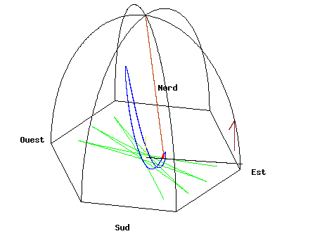
- Français : Animation du pendule de Foucault du Panthéon de Paris. English: Animation of the Foucault Pendulum from the dome of the Panthéon in Paris. Deutsch: Animation des Foucault'schen Pendels in der Panthéon Halle in Paris
-
 Français : Vue standardEnglish: Standard viewDeutsch: Standardsicht
 -
 Français : Vue du plan d'oscillationEnglish: View from the oscillation planeDeutsch: Sicht von dem Oszillationsplan
 -
 Français : Vue du soleilEnglish: View from the sunDeutsch: Sicht von der Sonne
 -
 Français : Notes pour la compréhension du programme de calcul du pendule de Foucault vu du SoleilEnglish: Notations used for the Pendulum animations, especially for the view from the sun.Deutsch: Verwendete Bezeichnungen für die Pendel-Animationen, insbesondere für die Sicht von der Sonne.
Summary
| Description |
Français : Animation d'un pendule de Foucault de 67 mètres qui serait laché au Panthéon de Paris à une distance de 50,25 mètres (3/4 de sa longueur) à l'est du centre de la coupole. Une corde permet de tendre le fil et d'attendre la fin des oscillations du cable. Puis on brûle la corde et ainsi le pendule est libéré avec une vitesse initiale nulle. La rotation de la Terre est également exagérée et correspond à une rotation en 110 secondes afin de mieux comprendre la dynamique. Le pendule se dirige vers le point d'équilibre mais en raison de la rotation de la Terre, la force de Coriolis, perpendiculaire au déplacement et proportionnelle à la vitesse du pendule (trace rouge), dévie le pendule vers le nord et le pendule évite ainsi un poteau central (qui n'existe pas car il devrait être extrêmement fin dans le cas d'une rotation en 24 heures). A l'opposé du point de lâcher, la vitesse du pendule s'annule ainsi que la force de déviation et le pendule repart dans l'autre sens en effectuant un point de rebroussement au sol (trace verte). La vitesse étant inversée, la force de Coriolis dévie le pendule vers le sud et le pendule passe au sud de sa position d'équilibre. Après une oscillation complète, le pendule ne revient donc pas à son point de lacher initial mais il a tourné d'un certain angle. Cet angle est néanmoins plus faible que la rotation de la Terre durant cette période d'oscillation et est proportionnel à l'inverse du sinus de la latitude. La rotation du plan d'oscillation est visualisé par la trace bleue. On remarque que cette ellipse tourne en effet moins vite que l'ombre du poteau central. Dans cet exemple, le pendule est lâché à midi un jour d'équinoxe, le soleil se couche donc exactement à l'ouest 6 heures après le lâcher. Le programme de l'animation Gnuplot est fourni (sous licence GPL) English: Animation of a fictitious pendulum of Foucault of 67 meters released at a distance of 50,25 meters (3/4 its length) in the east with a null speed. The rotation of the Earth is also exaggerated and corresponds to a rotation in 110 seconds. It corresponds to the view taken from the plane of oscillations: the terrestrial reference frame thus turns. But the shadow of a stick added at the center for ease of comprehension, rotates faster than the plane of oscillations. In this pseudo plan, the trace is not linear but corresponds to an ellipse. In this illustration, the pendulum is launched at noon at equinox. Thus the sun set is exactly six hours after the launch. Source of the Gnuplot animation is provided (GPL) Deutsch: Animation eines fiktiven Pendels von Foucault von 67 Metern Länge, das an einer Distanz von 50,25 Metern (3/4 seiner Länge) im Osten mit Null-Geschwindigkeit gestartet wurde. Die Rotation der Erde wird ebenfalls übertrieben und entspricht einer Umdrehung in 110 Sekunden. Diese Sicht ist von dem Oszillationsplan genommen: das Erdbezugssystem dreht sich also. In diesem Pseudoplan ist die Vorzeichnung am Boden nicht linear, sondern entspricht einer Ellipse. Der Quellcode der Gnuplot-Animation ist angegeben (GPL). |
| Date | |
| Source | Own work |
| Author | Nbrouard |
| Other versions |
 , ,  , ,  and other languages. and other languages.  |
Français : Le programme est décomposé en deux fichiers, foucault-anim.gp et foucault-iter.gp . Il suffit de compiler par une commande du genre :
gnuplot foucault-anim.gp pour obtenir le fichier .gif . Se reporter au programme pour les paramètres. En particulier fixe=0 donne le fichier anim.gif, fixe=1 le fichier rotz.gif et fixe=2 le fichier soleil.gif .
- Le logiciel libre Gnuplot fonctionne sous tous les systèmes d'exploitation. Pour obtenir les fonctionnalités des fichiers gif animés, il faut néanmoins utiliser une version 4.2 ou 4.3 qu'on peut trouver sur le CVS.
- Se reporter également à la page http://fr.wikipedia.org/w/index.php?title=Pendule_de_Foucault&oldid=15105524 pour les équations du mouvement du pendule.
- Pour le calcul de l'ombre du poteau central, voir les notes manuscrites Image:Foucault-solaire-ecliptique-notes.jpg qui peuvent aider à la compréhension des notations.
- Pour le calcul de la corde vibrante, il s'agit d'une simple sinusoïde et on peut se reporter à la page de Wikipédia sur les ondes sur une corde vibrante.
- Si vous voulez comprendre comment faire une animation plus simple du pendule, vous devez plutôt vous reporter aux toutes premières versions de cette animation en consultant l'historique de cette page. A moins d'une erreur, vous devriez trouver le fichier .gif correspondant dans l'historique des uploads.
- Si vous voulez améliorer le graphique, prière de respecter la licence GPL et d'indiquer votre nom, de décrire vos modifications et d'incrémenter le numéro de version.
English: The programme consists in two files foucault-anim.gp and foucault-iter.gp. In order to get one animated gif, just do the command:
gnuplot foucault-anim.gp
- Look at the section concerning the parameters to get a specific gif (anim for fixe=0, rotz for fixe=1 or soleil for fixe=2).
- Gnuplot is an open source software which runs on any operating system. But in order to produce animated gif images, you need to download a version 4.2 or above from the CVS tree.
- Please refer to http://fr.wikipedia.org/w/index.php?title=Pendule_de_Foucault&oldid=15105524 for the main equations of the pendulum.
- For the computation of the shadow of the central stick according to day, time, latitude, please refer to the manuscript Image:Foucault-solaire-ecliptique-notes.jpg which could help understanding the parameters and notations used.
- For the waving cable, I simply used a sine equation which came from the Wikipedia French page on the vibrating string.
- If you are interested in how to create simpler animation using gnuplot, the suggestion is to run a former version of this page (in the history). You should find the corresponding gif file in the history of the uploads.
- If you want to improve the graphics, or add legend for other languages, please respect the GPL licence by adding your name, describing the changes and incrementing the version number.
Source du programme GNUPLOT sous licence GPL
Foucault-anim.gp
Gnuplot source
reset
set ter x11 # or windows on Windows
# Programme Gnuplot foucault-anim.gp, ne fonctionne qu'avec une version >=4.2 et une libgd récente
# Nbrouard 7 mars 2007 v1.0 Sous licence GPL. GNU General Public License
# Nbrouard 12 mars 2007 v1.1
#             Ajout de l'ellipse et simplification des équations
# Nbrouard 14 mars 2007 v1.2
#             Ajout du fil du pendule.
# Nbrouard 16 mars 2007 v1.4
#             Suppression des axes et ajout d'une coupole
#             Indication pour le traitement des caractères unicode UTF-8
# Nbrouard 21 mars 2007 v1.5
#             Ajout gifsicle pour réduire la taille.
# Nbrouard 7 avril 2007 v1.6
#             Ajout d'un poteau central, sorte de cadran solaire vertical,
#             dont l'ombre tourne plus vite que le plan d'oscillation
# Nbrouard 7 avril 2007 v1.7
#             Ajout d'une troisième vue depuis le soleil
# Nbrouard 12 avril 2007 v1.8
#             Ajout d'une corde pour tendre le pendule loin de son point
#             d'équilibre. On attend la fin des oscillations du cable puis on
#             brûle la corde qui libère le pendule.
# Nbrouard 6 novembre 2010 v1.9
#             According to http://commons.wikimedia.org/wiki/Category:Animated_gifs_exceeding_the_12.5MP_limit
#             the thumbnails stopped to be animated because the original files were 640x480 with 81 frames = 24.9MP.
#             Now, I reduced to 448x336 x 81 = 12.2MP below the limit of 12.5MP
# Dernière version sous http://commons.wikimedia.org/wiki/Image:Foucault-rotz.gif
g=9.81 # gravité g/s2
l=67.   # longueur du pendule en mètres
omega=sqrt(g/l)

# Choisir la vitesse de rotation de la Terre
Omega=2.*pi/24./3600. # Rotation de la Terre, 24 heures par jour
Omega=2.*pi/(23.+(56./60.))/3600. # Rotation de la Terre, 23h56 jour sidéral (pour le 3e dessin)
Omega=2.*pi/3600.*60. # Rotation très rapide en 1/60e d'heure pour un dessin
Omega=2.*pi/3600./24.*24.*60./1.5 # Rotation très rapide en 2/3*1/60e d'heure 90 secondes pour le premier dessin
Omega=2.*pi/3600./24.*24.*60./3.5 # Rotation très rapide en 3.5 1/60e d'heure soit 110 secondes pour le second dessin
print "Période de la Terre 2.*pi/Omega= ",2.*pi/Omega, " secondes"

theta=(48.+52./60.)/360*2.*pi   # latitude de 48 degrés 52 minutes
omegz=sqrt(omega*omega+Omega*Omega*sin(theta)*sin(theta))

complex(x,y)=x*{1,0}+y*{0,1} # fonction utile

# cas où le pendule est propulsé du centre avec une vitesse de 2m/s (cas irréaliste non dessiné)
z0={0,0}
vz=2         # Si propulsé au centre avec une vitesse de 2 m/s
zp0=complex(vz,0)

# cas 'historique' où le pendule est lancé sans vitesse
#   initiale à z0 mètres à l'est du centre.
z0={6.,0}  # pour le 3e dessin
z0=l*3./4.*{1,0}  # pour les premier et second dessins
zp0={0,0}
print "Vitesse initiale ",zp0

c1=z0/2.*(1+Omega/omegz*sin(theta))*{1,0}-zp0/2./omegz*{0,1}
c2=z0/2.*(1-Omega/omegz*sin(theta))*{1,0}+zp0/2./omegz*{0,1}
unset label
eix(x)=cos(x)*{1,0}+sin(x)*{0,1}
#z(t)=c1*eix(-(Omega*sin(theta)-omegz)*t) + c2*eix(-(Omega*sin(theta)+omegz)*t)
z(t)=eix(-(Omega*sin(theta))*t)*(z0*(cos(omegz*t)*{1,0}+Omega*sin(theta)/omegz*sin(omegz*t)*{0,1})+zp0/omegz*sin(omegz*t))

set parametric
# Trace dans le pseudo plan d'oscillation (pas dessiné)
#plot real(c1*eix(omegz*t)+c2*eix(-omegz*t)), imag(c1*eix(omegz*t)+c2*eix(-omegz*t))
#plot [t=0:3.65*2.*pi/omegz] [-abs(z0):abs(z0)] [-abs(z0):abs(z0)] real(z(t)),imag(z(t))
h(t)=-sqrt(l*l-abs(z(t))*abs(z(t)))+l
hz=h(0)

# La coupole du Panthéon : nombre d'ogives 3 par défaut
# Il faut la tracer en paramétrique pour t variant de O à tf.
nogives=3.
spx(t,tf)= l*(cos(floor(t/tf*nogives)*pi/nogives)*cos(t/tf*pi*nogives))
spy(t,tf)= l*(sin(floor(t/tf*nogives)*pi/nogives)*cos(t/tf*pi*nogives))
sph(t,tf)= l*abs(sin(t/tf*pi*nogives))
#sph(t,tf)= l*abs(sin((abs((t-tf/nogives))/tf*nogives<1.e-2?pi*nogives:t/tf*nogives*pi)))

# Le fil du pendule
px(t,tf)= t/tf*real(z(tf))
py(t,tf) =t/tf*imag(z(tf))
ph(t,tf) =l+t/tf*(h(tf)-l)
# L'oscillation du fil du pendule (avant le lancement)
nonde=2.
bonde=2.
T=23
mu=1
v=sqrt(T/mu)
onde(x,t)=bonde*sin(nonde*pi*x/l)*cos(nonde*pi*v*t/l)
tondmax=l/v/nonde; tondmin=l/v/nonde/2.;tond=tondmin/2.
print "tondmax=",l/v/nonde," tondmin=",l/v/nonde/2.
xonde(t,tf,ti)=t/tf*l*real(z(tf))/l+(l-h(tf))/l*onde(t/tf*l,ti)
yonde(t,tf,ti)=0.
zonde(t,tf,ti)=l-t/tf*(l-h(tf))+real(z(tf))/l*onde(t/tf*l,ti);

# La corde qui retient le pendule et doit être brûlée.
a=2. # 20 centimètre de rayon pour le pendule lui-même
eta=pi/20. # a ajuster pour le graphique.
xcorde(t,tf)=z0+a*(sin(eta)*(1.-t/tf)+t/tf/sin(eta))
ycorde(t,tf)=a*cos(eta)*(1.-t/tf)

#--- Paramètres
#   Langues
lang="de"
lang="en"
lang="fr" # par défaut

#   Type de repère
fixe=0 # Dessin dans le repère terrestre : foucault-anim.gif
fixe=1 # Dessin dans le plan du pendule : foucault-rotz.gif
#fixe=2  # Vue du soleil : foucault-soleil.gif

#   Taille des fichiers animés
thumb=-1 # X11 or Win
thumb=0 # 448x336
#thumb=1 # 180x135 Miniatures par défaut de Wikipédia

split=1  # Si on souhaite des fichiers images séparés (dans un sous-répertoire)
split=0

# Le cadran solaire
#splot [t=0:2*pi] [:] [-2*pi:2*pi] [-2*pi:2*pi] 0.,0.,t with line lt 7, cos(psi)*t,sin(psi)*t,0 with line lt -1

epsilona=-(23./360.+26./360./60.)*2.*pi # angle apparent du zenith avec l'étoile polaire.
# 23°26' été ou hiver
epsilona=0./360.*2.*pi # angle apparent du zenith avec l'étoile polaire. Il dépend
# de la saison. Il vaut 0 pour les équinoxes, positif en été et négatif en hiver

htig=10. # hauteur de la tige en mètres

heure=(6.-12.)/24*2.*pi # 6 heures (ombre infinie aux équinoxes)
heure=(12.-12.)/24*2.*pi # Midi en radian

#-- Fin des paramètres
# theta-epsilona = angle du zenith avec les rayons de soleil à midi
# phi angle du zenith avec les rayons de soleil à l'heure h
phi(heure)=acos((cos(theta)*cos(epsilona)*cos(heure)+sin(theta)*sin(epsilona)))
X(heure)=cos(epsilona)*sin(heure)
Y(heure)=sin(theta)*cos(epsilona)*cos(heure)-cos(theta)*sin(epsilona)
Z(heure)=cos(theta)*cos(epsilona)*cos(heure)+sin(theta)*sin(epsilona)
#print X(heure)*X(heure)+Y(heure)*Y(heure)+Z(heure)*Z(heure) # vaut 1
#heurefin=heure+Omega*tf # en radian
debjour=acos(-tan(theta)*tan(epsilona))*24./2./pi-12. # Heure de début du jour ou fin du jour pour phi=pi/2
#splot [t=0:2*pi] [:] [-3*pi:3*pi] [-3*pi:3*pi] 0.,0.,htig*t/2./pi with line lt 7, X(heure)*htig*t/2./pi*tan(phi),Y(heure)*htig*t/2./pi,0 with line lt -1

# Pour traiter des caractères UTF-8, il faut obtenir par exemple des polices TrueType
# voir le site http://corefonts.sourceforge.net/
# Dans ce cas on peut faire set ter gif font "arial" 14 mais il faut
# que l'environnement GDFONTPATH pointe sur le répertoire TrueType :export GDFONTPATH="/usr/share/fonts/msttcorefonts/"
# export GNUPLOT_DEFAULT_GDFONT="arial"

if(lang ne "fr") ficlang=sprintf("-%s",lang); else ficlang="";
if (lang eq "de") Est="Osten"; Ouest="Westen"; Nord="Norden"; Sud="Süden"; \
else if (lang eq "en") Est="East";  Ouest="West"; Nord="North"; Sud="South"; \
else Est="Est"; Ouest="Ouest"; Nord="Nord"; Sud="Sud";

unset label
set label Est at l*1.2,0,0 center
set label Ouest at -l*1.2,0,0 center
set label Nord at 0,l*1.2,0 center
set label Sud at 0,-l*1.2,0 center
#set xlabel "Ouest <-> Est en metres"
#set ylabel "Sud <-> Nord en metres"

#set samples 100
set xyplane at 0
#set size 0.75,1 # aspect circulaire 480/640=0.75 # Merci à Michel Barbetorte 07/03/07
rotationz=28
rotationz=0
rotationx=50
#set view rotationx,rotationz,1,1.5
set view rotationx,rotationz,1,1.0
# dessin à l'écran pour voir
splot [t=0:3.65*2.*pi/omegz] [:] [-abs(z0):abs(z0)] [-abs(z0):abs(z0)] [0:l] real(z(t)),imag(z(t)),((t<pi/omegz)&&(t>0)?h(t):1/0) with lines lt palette , real(z(t)),imag(z(t)),0 with lines

unset title
unset key
unset xtics
unset ytics
unset ztics
set border 0
set size square
set size 1.3,1.3
set size 1.5,1.5
set size 1.54,1.54
#set size 0.75,1
#set size 1.0,1.0
set origin -0.4,-0.15
#set origin -0.4,-0.15
 set origin -0.2,-0.15
#set origin 0.,0.
 sampbase=700
set samples sampbase
n=24
tdelta=2.*pi/omegz/n
tfin=12*2.*pi/omegz
tfin=3*2.*pi/omegz
#tfin=pi/omegz
limit_iterations=9*n
#limit_iterations=6
#limit_iterations=13
tmin=1.e-3
tdeb=tdelta
tdeb=tmin
iteration_count=0
if(fixe==1) rotationz=75.; else  rotationz=28.
set view rotationx,rotationz,1,1.0
#set ter gif size 640,480 large animate optimize
# set ter gif animate optimize size 640,480 \
#                         xffffff x000000 x404040 \
#                         xff0000 xffa500 x66cdaa xcdb5cd \
#                         xadd8e6 x0000ff xdda0dd x9500d3    # defaults

if(thumb==1) xpix=180;ypix=135; else xpix=448;ypix=336;
#if(thumb==1) xpix=180;ypix=135; else xpix=640;ypix=480;
#if(thumb==1) xpix=180;ypix=135; else xpix=540;ypix=405;
if(fixe==1) tfixe="rotz";else if (fixe==2) tfixe="soleil"; else tfixe="anim";
set size 1.54*ypix/xpix,1.54
iteration_count=0
if(thumb==1) labpix=sprintf("%dx%d-",xpix,ypix); else labpix="";
if(split != 1) ficsortie=sprintf("%sfoucault-%s%s.gif",labpix,tfixe,ficlang) # else voir dans la boucle

if(thumb==-1) set ter x11; set out; else if(split==1) set ter gif animate optimize size xpix,ypix xffffff x000000 xa0a0a0 xff0000 x00c000 x0080ff xc000ff x00eeee ; set out; else set ter gif animate optimize size xpix,ypix  xffffff x000000 xa0a0a0 xff0000 x00c000 x0080ff xc000ff x00eeee; set out ficsortie;
show ter
show output

rotationdynz=rotationz/360.*2.*pi
if(fixe==1) rotationzinc=-tdelta*Omega*sin(theta); else rotationzinc=0 # Pour fixe==2 voir foucault-rot-ellipse.gp car la rotation est plus complexe
debut=1
call "foucault-iter.gp" "Rotationz" rotationzinc split fix # en fait les valeurs des variables sont passées par défaut
set ter X11
set out
replot
# Gnuplot 2.3 rc4 semble moins bien optimser que gifsicle ou Gimp pour réduire sa taille.
# Ici on a fait :
#! gifsicle  -b foucault-anim.gif -d150 '#6' -d150 '#7' -d50 '#8'
#! gifsicle -O2 -k8 foucault-anim.gif -o  foucault-anim-O2-k8.gif
###! gifsicle  -b foucault-rotz.gif -d150 '#6' -d150 '#7' -d50 '#8'
###! gifsicle -O2 -k8 foucault-rotz.gif -o  foucault-rotz-O2-k8.gif
#! gifsicle -O2 -k8 foucault-soleil.gif -o  foucault-soleil-O2-k8.gif
# Fin
Foucault-iter.gp
Nous avons besoin d'un programe d'itération (Foucault-iter.gp) pour faire plusieurs images:
Gnuplot source
# Foucault-iter.gp
# Version 1.8 du 12 avril 2007
# Dernière version sous http://commons.wikimedia.org/wiki/Image:Foucault-rotz.gif
if(split==1) ficsortie=sprintf("foucault-%s%s/%sfoucault-%s%s-%d.gif",tfixe,ficlang,labpix,tfixe,ficlang,iteration_count);set out ficsortie
print "Fichier Rotationz=$0 rotationzinc=$1 split=$2 ficsortie=",ficsortie
print "1-rotationdynz=",rotationdynz, " deg=", rotationdynz/2./pi*360.
rotationdynz=rotationdynz+$1
rotationdyndegz=rotationdynz/2./pi*360.
rotationdyndegz=rotationdyndegz -int(rotationdyndegz/360.)*360.
if(rotationdyndegz<0) rotationdyndegz=rotationdyndegz+360.
print "2-rotationdynz=",rotationdynz, " deg=", rotationdyndegz
if(fixe==2) set view phi(heure+Omega*tdeb)/2./pi*360.,360.-90.+atan(Y(heure+Omega*tdeb)/X(heure+Omega*tdeb))/2./pi*360.,1.,real(ypix)/real(xpix); else set view ,rotationdyndegz,,
iteration_count=iteration_count+1
if(tdeb/tdelta>sampbase) set samples tdeb*sampbase/tdelta
znonrot(t)=eix(-Omega*sin(theta)*(tdeb-t))*z(t)
print "iteration_count in ", iteration_count," limit_iterations ", limit_iterations, " tdeb ",tdeb," xnonrot(tdeb) ", real(znonrot(tdeb))," ynonrot(tdeb) ",imag(znonrot(tdeb))

if(debut==1 )ti=0.;splot [t=0:tdeb] [:] [-l:l] [-l:l] [0:l] \
     spx(t,tdeb),spy(t,tdeb),sph(t,tdeb) not with lines lc rgb 'black', \
     spx(t,tdeb),-spy(t,tdeb),sph(t,tdeb) not with lines lc rgb 'black', \
     z0+a*cos(t/tdeb*(pi+2*eta)+pi/2.-eta),a*sin(t/tdeb*(pi+2*eta)+pi/2.-eta),h(0) not with lines lc rgb 'brown', \
     xcorde(t,tdeb), ycorde(t,tdeb),h(0) not with lines lc rgb 'brown', \
     xcorde(t,tdeb),-ycorde(t,tdeb),h(0) not with lines lc rgb 'brown', \
     xonde(t,tdeb,ti),yonde(t,tdeb,ti),zonde(t,tdeb,ti) not with lines lt 6;
if(debut==1 )ti=1.*tond;splot [t=0:tdeb] [:] [-l:l] [-l:l] [0:l] \
     spx(t,tdeb),spy(t,tdeb),sph(t,tdeb) not with lines lc rgb 'black', \
     spx(t,tdeb),-spy(t,tdeb),sph(t,tdeb) not with lines lc rgb 'black', \
     z0+a*cos(t/tdeb*(pi+2*eta)+pi/2.-eta),a*sin(t/tdeb*(pi+2*eta)+pi/2.-eta),h(0) not with lines lc rgb 'brown', \
     xcorde(t,tdeb), ycorde(t,tdeb),h(0) not with lines lc rgb 'brown', \
     xcorde(t,tdeb),-ycorde(t,tdeb),h(0) not with lines lc rgb 'brown', \
     xonde(t,tdeb,ti),yonde(t,tdeb,ti),zonde(t,tdeb,ti) not with lines lt 6;
if(debut==1 )ti=2.*tond;splot [t=0:tdeb] [:] [-l:l] [-l:l] [0:l] \
     spx(t,tdeb),spy(t,tdeb),sph(t,tdeb) not with lines lc rgb 'black', \
     spx(t,tdeb),-spy(t,tdeb),sph(t,tdeb) not with lines lc rgb 'black', \
     z0+a*cos(t/tdeb*(pi+2*eta)+pi/2.-eta),a*sin(t/tdeb*(pi+2*eta)+pi/2.-eta),h(0) not with lines lc rgb 'brown', \
     xcorde(t,tdeb), ycorde(t,tdeb),h(0) not with lines lc rgb 'brown', \
     xcorde(t,tdeb),-ycorde(t,tdeb),h(0) not with lines lc rgb 'brown', \
     xonde(t,tdeb,ti),yonde(t,tdeb,ti),zonde(t,tdeb,ti) not with lines lt 6;
if(debut==1 )ti=3.*tond;splot [t=0:tdeb] [:] [-l:l] [-l:l] [0:l] \
     spx(t,tdeb),spy(t,tdeb),sph(t,tdeb) not with lines lc rgb 'black', \
     spx(t,tdeb),-spy(t,tdeb),sph(t,tdeb) not with lines lc rgb 'black', \
     z0+a*cos(t/tdeb*(pi+2*eta)+pi/2.-eta),a*sin(t/tdeb*(pi+2*eta)+pi/2.-eta),h(0) not with lines lc rgb 'brown', \
     xcorde(t,tdeb), ycorde(t,tdeb),h(0) not with lines lc rgb 'brown', \
     xcorde(t,tdeb),-ycorde(t,tdeb),h(0) not with lines lc rgb 'brown', \
     xonde(t,tdeb,ti),yonde(t,tdeb,ti),zonde(t,tdeb,ti) not with lines lt 6;
if(debut==1 )ti=4.*tond;splot [t=0:tdeb] [:] [-l:l] [-l:l] [0:l] \
     spx(t,tdeb),spy(t,tdeb),sph(t,tdeb) not with lines lc rgb 'black', \
     spx(t,tdeb),-spy(t,tdeb),sph(t,tdeb) not with lines lc rgb 'black', \
     z0+a*cos(t/tdeb*(pi+2*eta)+pi/2.-eta),a*sin(t/tdeb*(pi+2*eta)+pi/2.-eta),h(0) not with lines lc rgb 'brown', \
     xcorde(t,tdeb), ycorde(t,tdeb),h(0) not with lines lc rgb 'brown', \
     xcorde(t,tdeb),-ycorde(t,tdeb),h(0) not with lines lc rgb 'brown', \
     xonde(t,tdeb,ti),yonde(t,tdeb,ti),zonde(t,tdeb,ti) not with lines lt 6;
if(debut==1 ) ti=5.*tond;splot [t=0:tdeb] [:] [-l:l] [-l:l] [0:l] \
     spx(t,tdeb),spy(t,tdeb),sph(t,tdeb) not with lines lc rgb 'black', \
     spx(t,tdeb),-spy(t,tdeb),sph(t,tdeb) not with lines lc rgb 'black', \
     z0+a*cos(t/tdeb*(pi+2*eta)+pi/2.-eta),a*sin(t/tdeb*(pi+2*eta)+pi/2.-eta),h(0) not with lines lc rgb 'brown', \
     xcorde(t,tdeb), ycorde(t,tdeb),h(0) not with lines lc rgb 'brown', \
     xcorde(t,tdeb),-ycorde(t,tdeb),h(0) not with lines lc rgb 'brown', \
     xonde(t,tdeb,ti),yonde(t,tdeb,ti),zonde(t,tdeb,ti) not with lines lt 6;
if(debut==1 )ti=6*tond;splot [t=0:tdeb] [:] [-l:l] [-l:l] [0:l] \
     spx(t,tdeb),spy(t,tdeb),sph(t,tdeb) not with lines lc rgb 'black', \
     spx(t,tdeb),-spy(t,tdeb),sph(t,tdeb) not with lines lc rgb 'black', \
     X(heure+Omega*tdeb)/Z(heure+Omega*tdeb)*htig*t/tdeb,Y(heure+Omega*tdeb)/Z(heure+Omega*tdeb)*htig*t/tdeb,0 with line lt -1, \
     0.,0., htig*t/tdeb with line lt 7, \
     z0+a*cos(t/tdeb*(pi+2*eta)+pi/2.-eta),a*sin(t/tdeb*(pi+2*eta)+pi/2.-eta),h(0) not with lines lc rgb 'brown', \
     xcorde(t,tdeb), ycorde(t,tdeb),h(0) not with lines lc rgb 'brown', \
     xcorde(t,tdeb),-ycorde(t,tdeb),h(0) not with lines lc rgb 'brown', \
     xonde(t,tdeb,ti),yonde(t,tdeb,ti),zonde(t,tdeb,ti) not with lines lt 6;
if(debut==1) replot xcorde(t,tdeb),-ycorde(t,tdeb),((tdeb*0.4<t)&&(t<=tdeb*0.6)?h(t):1/0) not with lines lc rgb 'red' lw 3 ;
if(debut==1) replot xcorde(t,tdeb),-ycorde(t,tdeb),((tdeb*0.3<t)&&(t<=tdeb*0.7)?h(t):1/0) not with lines lc rgb 'red' lw 3, \
    xcorde(t,tdeb),-ycorde(t,tdeb),((tdeb*0.4<t)&&(t<=tdeb*0.6)?h(t):1/0) not with lines lc rgb 'yellow' lw 4 ;
debut=0
     if (((!limit_iterations) || (iteration_count<=limit_iterations)) && (tdeb <= tfin)) \
   print "iteration_count loop ",iteration_count; \
   splot [t=0:tdeb] [:] [-l:l] [-l:l] [0:l] \
     xcorde(tdeb,tdeb),0., (1.-(xcorde(tdeb,tdeb)-xcorde(t,tdeb))/20.)*h(0) not with lines lc rgb 'brown', \
     xcorde(tdeb,tdeb)*(1.-(xcorde(tdeb,tdeb)-xcorde(t,tdeb))/200.),0., (1.-(xcorde(tdeb,tdeb)-xcorde(t,tdeb))/60.)*h(0) not with lines lc rgb 'brown', \
     real(z(t)),imag(z(t)),0 not with lines lc rgb 'green', \
     real(znonrot(t)),imag(znonrot(t)),((0<=t)&&(t<=tdeb)?h(t):1/0) not with lines lc rgb 'blue', \
     px(t,tdeb),py(t,tdeb),((0<=t)&&(t<=tdeb)?ph(t,tdeb):1/0) not with lines lt 6, \
     real(z(t)),imag(z(t)),((tdeb-tdelta/2.<t)&&(t<=tdeb)?h(t):1/0) not with lines lc rgb 'red' lw 3, \
     spx(t,tdeb),spy(t,tdeb),sph(t,tdeb) not with lines lc rgb 'black', \
     spx(t,tdeb),-spy(t,tdeb),sph(t,tdeb) not with lines lc rgb 'black', \
     X(heure+Omega*tdeb)/Z(heure+Omega*tdeb)*htig*t/tdeb,Y(heure+Omega*tdeb)/Z(heure+Omega*tdeb)*htig*t/tdeb,0 with line lt -1, \
     0.,0., htig*t/tdeb with line lt 7; \
     tdeb=tdeb+tdelta; \
   print (iteration_count+0.1-0.1)/limit_iterations*100, " pour cent"; \
   print "heure = ", (heure+Omega*tdeb)/2./pi*24.+12.," phi(heure+Omega*tdeb)=",phi(heure+Omega*tdeb)/2./pi*360.,360.-90.+atan(Y(heure+Omega*tdeb)/X(heure+Omega*tdeb))/2./pi*360. ;\
reread
  #pause mouse any "Any key or button will terminate" ;
Licensing
Same licenses than other three images of the gallery. It means Creative Common Share Alike (3 or 2) for texts (replacing GFDL) and images, GPL for program code.
| This file is licensed under the Creative Commons Attribution-Share Alike 3.0 Unported license. | ||
| ||
| This licensing tag was added to this file as part of the GFDL licensing update. |
File history
Click on a date/time to view the file as it appeared at that time.
| Date/Time | Thumbnail | Dimensions | User | Comment | |
|---|---|---|---|---|---|
| current | 01:23, 30 January 2013 | | 448 × 336 (264 KB) | TMg | Missing lines and text added; last frame moved to first position for print and browsers without or disabled animations |
| 17:58, 6 November 2010 |  | 448 × 336 (273 KB) | Nbrouard | Image is reduced from 640x480 to 540x405 to fit the new 12.5MP limit with 81 frames to get animated thumbnails: http://commons.wikimedia.org/wiki/Category:Animated_gifs_exceeding_the_12.5MP_limit | |
| 20:05, 21 November 2009 |  | 640 × 480 (391 KB) | Nbrouard | This file was built in April 2007 like the ''anim'' and ''soleil'' files but never uploaded because its size was critical and thumbs took one week (yes) to be built: let see now how wikipedia improved its performance yet. | |
| 06:51, 7 April 2007 |  | 640 × 480 (372 KB) | Nbrouard | ||
| 11:28, 23 March 2007 |  | 640 × 480 (382 KB) | Nbrouard | ||
| 13:20, 16 March 2007 |  | 640 × 480 (393 KB) | Nbrouard | ||
| 20:15, 14 March 2007 |  | 640 × 480 (276 KB) | Nbrouard | ||
| 08:54, 12 March 2007 |  | 640 × 480 (457 KB) | Nbrouard | {{Information |Description= {{fr|Animation d'un pendule de Foucault de 67 mètres fictif laché à une distance de 50,25 mètres (3/4 de sa longueur) à l'est avec une vitesse nulle. La rotation de la Terre est également exagérée et correspond à une r | |
| 08:00, 7 March 2007 |  | 640 × 480 (412 KB) | Nbrouard | {{Information |Description= {{fr|Animation d'un pendule de Foucault de 67 mètres fictif laché à une distance de 50,25 mètres (3/4 de sa longueur) à l'est avec une vitesse nulle. La rotation de la Terre est également exagérée et correspond à une r |
File usage
The following 2 pages use this file:
Global file usage
The following other wikis use this file:
- Usage on ast.wikipedia.org
- Usage on bn.wikipedia.org
- Usage on ca.wikipedia.org
- Usage on cs.wikipedia.org
- Usage on cy.wikipedia.org
- Usage on de.wikipedia.org
- Usage on en.wikipedia.org
- Usage on en.wikibooks.org
- Usage on en.wiktionary.org
- Usage on es.wikipedia.org
- Usage on et.wikipedia.org
- Usage on fr.wikipedia.org
- Usage on ga.wikipedia.org
- Usage on hi.wikipedia.org
- Usage on ja.wikipedia.org
- Usage on ko.wikipedia.org
- Usage on lv.wikipedia.org
- Usage on ml.wikipedia.org
- Usage on pl.wikipedia.org
- Usage on sr.wikipedia.org
- Usage on zh.wikipedia.org